A graph consists of points — called nodes or vertices — connected by line segments — called edges.
The only library we will need for this tutorial is igraph:
library(igraph)
1. Directed graphs
A directed graph, where the edges indicate a one-way relationship between vertices, can be created from a data.frame that simply defines the edges:
edges_df <- data.frame(
  from = c('A', 'B'),
  to = c('B', 'C')
)
edges_df
#  from to
#1    A  B
#2    B  C

# create and plot igraph object
g = graph_from_data_frame(edges_df)
plot(g)
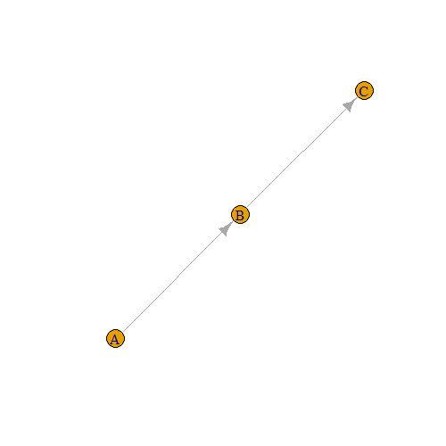
The function graph_from_data_frame() reads the data.frame row by row and creates a directed graph.
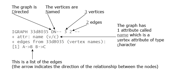
If we look inside the igraph object g we see the following:
print(g)
#IGRAPH 33d8035 DN-- 3 2 --
#+ attr: name (v/c)
#+ edges from 33d8035 (vertex names):
#[1] A->B B->C
Here’s a brief explanation of the output:
2. Undirected graphs
An undirected graph, where the edges have no direction, can be created using the same function but with the directed argument set to FALSE:
g = graph_from_data_frame(edges_df, directed = FALSE)
g
#IGRAPH b9d80a4 UN-- 3 2 --
#+ attr: name (v/c)
#+ edges from b9d80a4 (vertex names):
#[1] A--B B--C
The first line of the output states that the object is UN: an Undirected graph with Named vertices; and the last line uses “- -” instead of “->” to indicate an undirected relationship between the vertices.
plot(g)

2.a. Adjacency matrix
The adjacency matrix is a square matrix where the rows and columns are indexed by all the vertices of the graph and the values inside the matrix represent the relationship between them.
We can obtain the adjacency matrix of g by calling the function get.adjacency(g) or by simply typing g[]:
g[]
#3 x 3 sparse Matrix of class "dgCMatrix"
#  A B C
#A . 1 .
#B 1 . 1
#C . 1 .
The output is a sparse matrix where all zero values are replaced with a dot. We can transform this sparse matrix into an ordinary matrix by calling get.adjacency(g, sparse=FALSE) or as.matrix(g[]):
as.matrix(g[])
#  A B C
#A 0 1 0
#B 1 0 1
#C 0 1 0
A heatmap can help us visualize this matrix:
heatmap(as.matrix(g[]), Colv = NA, Rowv = NA, symm = TRUE)
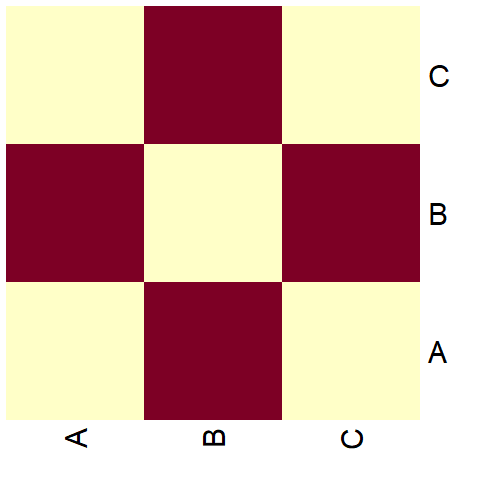
A red square indicates the presence of an edge between the corresponding vertices and a yellow one indicates the absence of an edge.
2.b. Isolated vertices
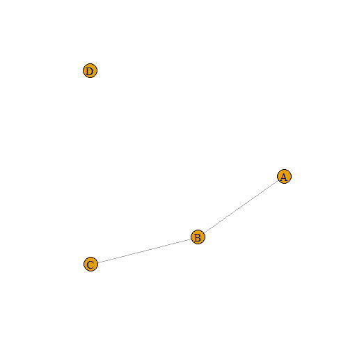
So far, we have been creating graphs using only a data.frame that defines the edges, but we haven’t discussed yet how to create a graph that contains an isolated vertex (one that is not linked to any other vertices).
In this case, we can provide the function graph_from_data_frame() another data.frame, vertices_df, that contains the names of all the vertices that should be included in the graph:
edges_df <- data.frame(
  from = c('A', 'B'),
  to = c('B', 'C')
)

vertices_df <- data.frame(
  names = c('A', 'B', 'C', 'D')
)

g = graph_from_data_frame(edges_df,
                          directed = FALSE,
                          vertices = vertices_df)
g
#IGRAPH 66c3ca4 UN-- 4 2 --
#+ attr: name (v/c)
#+ edges from 66c3ca4 (vertex names):
#[1] A--B B--C
Notice that the first line of the output says that now we have a graph with 4 vertices (A, B, C, and D) and 2 edges:
plot(g)
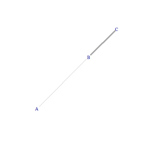
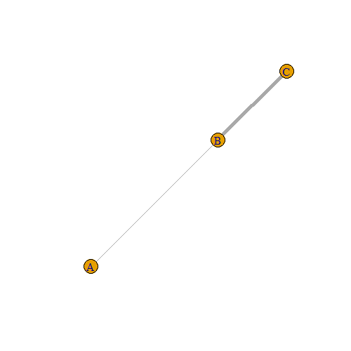
3. Weighted graphs
A weighted graph is one where each edge is associated with a weight value (a non-negative number) that represents, for example, its importance or its strength.
The function graph_from_data_frame() automatically creates a weighted graph by recognizing the presence of a variable called weight in the data.frame:
edges_df <- data.frame(
  from = c('A', 'B'),
  to = c('B', 'C'),
  weight = c(1, 5)
)
edges_df

g = graph_from_data_frame(edges_df, directed = FALSE)
g
#IGRAPH 6f1d96c UNW- 3 2 --
#+ attr: name (v/c), weight (e/n)
#+ edges from 6f1d96c (vertex names):
#[1] A--B B--C
Now the first line of the output indicates that the graph is UNW, meaning: Undirected, with Named vertices, and Weighted.
In order to plot this weighted graph, we have to specify that we want the edge.width to be equal to the weight variable:
plot(g, edge.width = edges_df$weight)
3.a. Adjacency matrix
heatmap(as.matrix(g[]), Colv = NA, Rowv = NA, symm = TRUE)
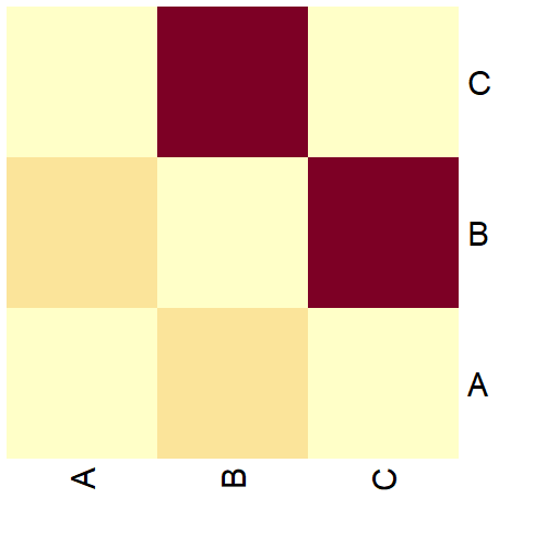
Now the heatmap of the adjacency matrix also represents the weights of the edges with a color gradient.
3.b. Other plotting options
We can separate the vertex labels and the vertex points in the plot by using the argument vertex.label.dist:
plot(g, vertex.label.dist = 2.5,
     edge.width = edges_df$weight)

Or we can keep only the vertex labels by setting vertex.shape = "none":
plot(g, vertex.shape = 'none',
     edge.width = edges_df$weight)