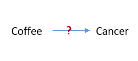
Suppose we want study whether coffee causes cancer, which we will represent as follows:
Randomizing people to either consume coffee or not for many years in order to study its effect on cancer is neither ethical nor practical. So we have to use an observational design, where we would have to deal with bias and confounding ourselves.
After collecting data, we decided to run the following regression model to study the effect of coffee on cancer:
Cancer = β0 + β1 Coffee + (other variables)??
The question is:
Which additional variables should we include (or avoid including) in our model in order for β1 to reflect a causal association between coffee and cancer and not just an association between the two?
In order for β1 to reflect a causal association, all other paths from coffee to cancer must be blocked i.e. coffee and cancer must be d-separated. In other words, all explanations other than the direct effect of coffee on cancer must be eliminated.
The 4 rules of D-separation can help us block these paths:
Rule #1: Conditioning on a confounder blocks the path between exposure and outcome
A confounder is a variable that represents a common cause of both the exposure and the outcome.
A confounder opens the path between exposure and outcome, therefore, when a confounder is present, we expect to find an association between exposure and outcome that is not causal in nature that can be mistaken for a causal one if we do not control for the confounder.
Let’s explain this statement by returning to our example above, and assuming that smoking can confound the relationship between Coffee and Cancer:
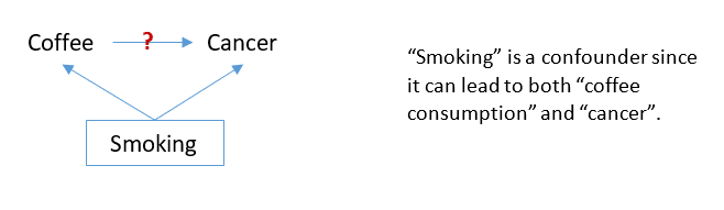
When a confounding variable exists, the β1 coefficient in the model “Cancer = β0 + β1 Coffee” may be statistically significant, although there is no causal relationship between the 2 variables.
By conditioning on the confounder (smoking), via stratification or via including it in the regression model, we block the path between the exposure (coffee) and the outcome (cancer).
Why?
Suppose that the variable smoking is binary:
- Non-smokers: 0
- Smokers: 1
For a given level of smoking, take smokers for example (where smoking = 1), studying the effect of coffee on cancer within this subgroup eliminates the effect of smoking (because it will be constant within the subgroup), and therefore, any association found between coffee and cancer will only be due to the causal effect of coffee on cancer.
This means that after including Smoking in the model above, the β1 coefficient in the model “Cancer = β0 + β1 Coffee + β2 Smoking” will only be statistically significant when there is a causal association between coffee and cancer.
BOTTOM LINE:
Rule #1: Include all common causes of the exposure and the outcome in your regression model in order to eliminate alternative explanations of the outcome due to confounding.
Rule #2: Conditioning on a mediator variable blocks the path between exposure and outcome
A mediator is a variable that lies on the causal path between an exposure and an outcome, that explains how the exposure affects the outcome.
In our example above, suppose that coffee leads to DNA damage, which in turn will lead to cancer. This will make DNA damage a mediator of the relationship between coffee and cancer:
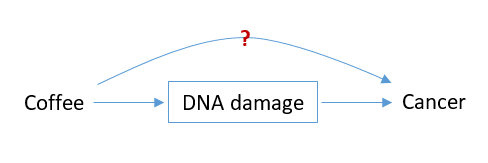
Suppose that we are interested in answering the question:
Does coffee have a direct effect on cancer? (that is not through DNA damage)
In order to answer this question, we need to study the effect of coffee on cancer for all levels of DNA damage. In other words, we need to condition on (or control for) DNA damage.
If after including DNA damage in the regression model “Cancer = β0 + β1 Coffee + β2 DNA damage”, the coefficient β1 is still statistically significant, this means that coffee has an effect on cancer irrespective of DNA damage.
BOTTOM LINE:
Rule #2: In order to study the direct effect of an exposure on an outcome, block other paths by conditioning on 1 mediator of each path.
Rule #3: Conditioning on a collider opens the path between exposure and outcome
A collider is a variable that represents a common effect of both the exposure and the outcome.
In our example, Anxiety is a collider since it is a common effect of both coffee and cancer:
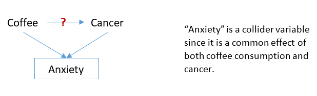
Conditioning on a collider leads to a spurious association between the exposure and the outcome.
Why?
For the sake of argument, suppose that anxiety can only be caused by either coffee or cancer. Now, let’s consider an individual who is highly anxious: If this person does not have cancer, then this would mean that his/her anxiety is probably due to coffee consumption, because something must have caused the anxiety after all.
Therefore, for a specific level of anxiety, knowing the value of the variable cancer, we can predict the value of coffee, and vice versa. This means that conditioning on anxiety leads to a non-causal association between coffee and cancer.
BOTTOM LINE:
Rule #3: Avoid including a collider in your regression model in order to avoid inducing a spurious association between the exposure and the outcome.
Rule #4: Conditioning on a descendent of a collider opens the path between exposure and outcome
A descendent of a collider is a variable that is caused by the collider.
In our example, Sleep problems can be considered a descendent of Anxiety:
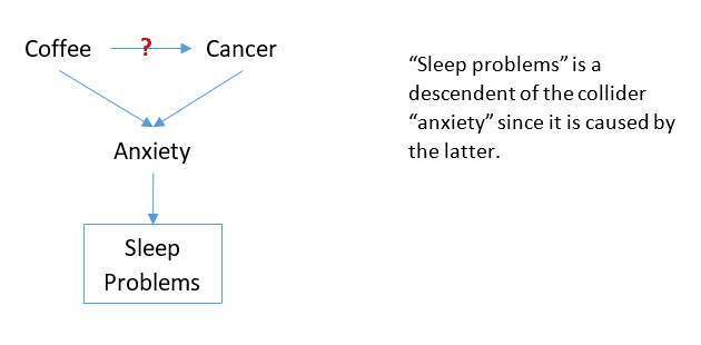
Controlling for sleep problems will induce a non-causal association between coffee and cancer. This is because the descendent of the collider is highly correlated with the collider variable, so that conditioning on the descendent of the collider has the same effect as conditioning on the collider.
BOTTOM LINE:
Rule #4: Avoid including the descendent of a collider in your regression model in order to avoid inducing a spurious correlation between the exposure and the outcome.
References
- Hernán MA, Robins JM. Causal Inference: What If. Boca Raton: Chapman & Hall/CRC; 2020.
- Pearl J, Glymour M, Jewell NP. Causal Inference in Statistics – A Primer. 1st edition. Wiley; 2016.