Interpret Linear Regression Output in R

Here’s an example of linear regression in R:

set.seed(1)

# simulating some fake data with a sample size of 100
x = rnorm(100)
z = sample(c(0,1), 100, replace = TRUE)
y = 0.4*x + 0.5*z + rnorm(100)

dat = data.frame(x = x, z = z, y = y)

# linear regression
summary(lm(y ~ x + z, data = dat))

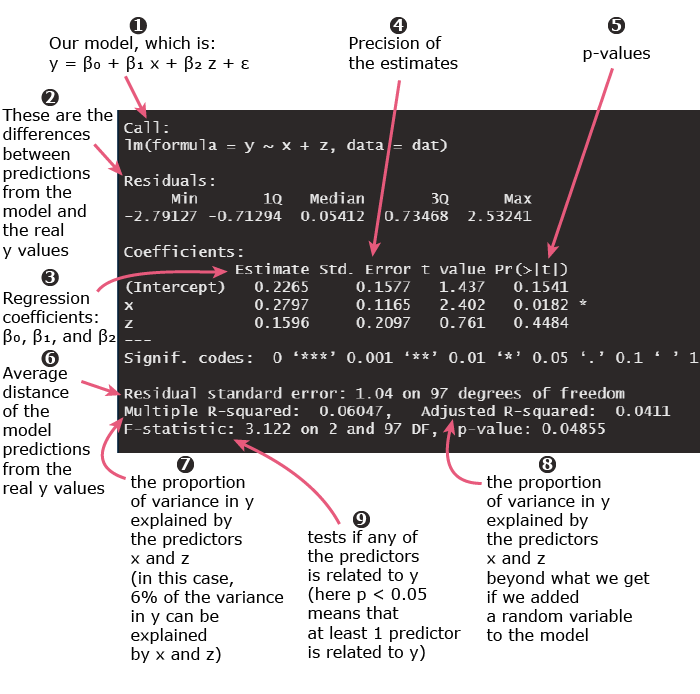
1. Linear regression equation

The formula \(y \sim x + z\) corresponds to the regression equation:

\(y = β_0 + β_1x + β_2z\)

where:

y is the response (also called outcome, or dependent variable)
x and z are the predictors (also called features, or independent variables)

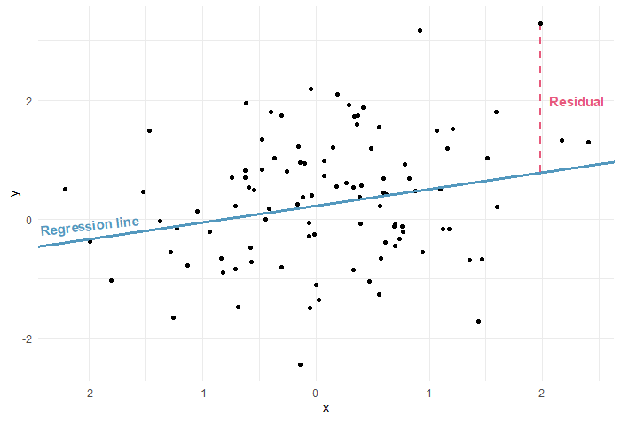
2. Residuals

The residuals are the difference between the regression line that we fitted (using the predictors x and z) and the real y values:

For linear regression, we need the residuals to be normally distributed.

The residuals table outputted by R can be used to quickly check if their distribution is symmetric (a normal distribution is symmetric and bell-shaped).

But instead of looking at raw numbers, I am going to use them to draw a boxplot (just because it is more visually appealing):

boxplot(model$residuals)

Output:

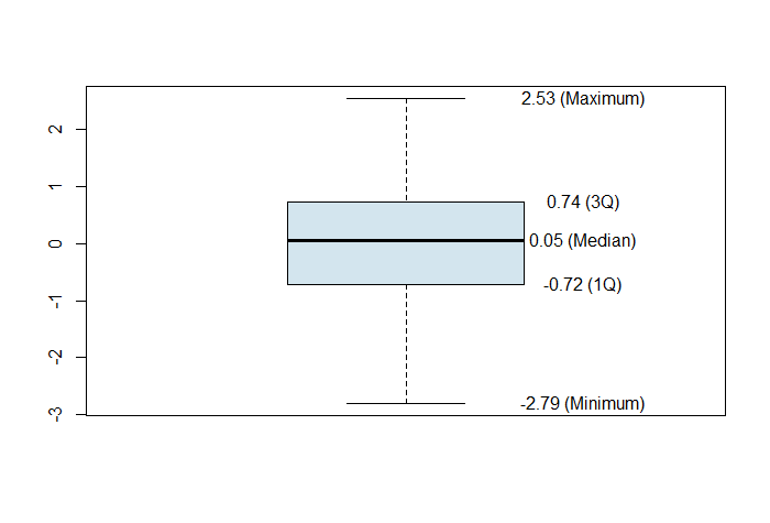
Since, the median is in the middle of the box and the whiskers are about the same length, we can conclude that the distribution of the residuals is symmetric.

Next, we can plot the histogram of the residuals or the normal Q-Q plot, or use a normality test to assess their normality.

3, 4, 5. Linear regression coefficients, standard errors, and p-values

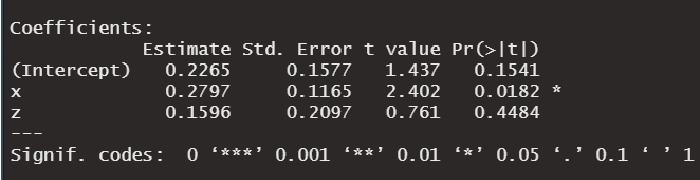
Estimate

This column contains the coefficients (β₀, β₁, and β₂) of each of the predictors in the equation:

\(y = β_0 + β_1x + β_2z\)

For example, β₁ = 0.2797 can be interpreted as follows:

After adjusting for z, β₁ is the expected difference in the outcome y for 2 groups of observations that differ by 1 unit in x.

(For more information, I have articles that cover how to interpret the linear regression intercept, how to interpret the linear regression coefficients for different types of predictors (categorical, numerical or ordinal), and how to interpret interactions in linear regression)

Std. Error

The coefficient’s standard error (SE) can be used to compute a confidence interval.

For example, for β₁ the 95% confidence interval is:

\(β_1 ± 2×SE(β_1)\)

replacing the numbers, we get:

\(95\% CI = [0.0467, 0.5127]\)

This puts lower and upper bounds on the effect of x on y.

The 95% confidence interval can be interpreted as follows:

We are 95% confident that the average difference in y between groups that differ by 1 unit in x is somewhere between 0.0467 and 0.5127.

t value

This is the coefficient divided by the standard error. It is useful to calculate the p-values for the coefficients.

Pr(>|t|)

This is the p-value associated with each coefficient.

A low p-value indicates that our results are so unusual assuming they were due to chance only, So, a low p-value is saying that: according to data from our sample, the regression coefficient is so high to be assuming that it is zero in the population data.

(I recommend this article on correct and incorrect interpretations of a p-value)

In general, we choose 0.05 to be the threshold for statistical significance. So, a p-value < 0.05 indicates statistical significance.

In our example above:

The coefficient of the variable x is associated with a p-value < 0.05, therefore, we can say that x has a statistically significant effect on y.

Signif. codes

The significance codes provide a quick way to check which coefficients in the model are statistically significant.

There are 5 options:

Symbol	Meaning
*******	0 < p-value < 0.001
**	0.001 < p-value < 0.01
*	0.01 < p-value < 0.05
.	0.05 < p-value < 0.1
	0.1 < p-value < 1

6. Residual standard error

The residual standard error is a way to assess how well the regression line fits the data. The smaller the residual standard error, the better the fit.

In our example, the residual standard error of 1.04 can be interpreted as follows:

The linear regression model predicts y values with an average error of 1.04 units.

Where do the 97 degrees of freedom come from?

The degrees of freedom df are the sample size minus the number of parameters that we are trying to estimate.

Since our sample size is 100 and we are estimating 3 parameters: β₀, β₁, and β₂, then, df = 100 – 3 = 97.

(For more information, I wrote a separate article on how to calculate and interpret the residual standard error)

7, 8. Multiple R-squared and adjusted R-squared

R-squared is another way to measure the quality of the fit of the linear regression model.

Multiple R-squared is the proportion of variance in y that can be explained by the predictors x and z.

In our case, multiple R-squared is 0.06047 or 6.047%, which means that x and z explain approximately 6% of the variance of y (and 94% is left unexplained).

(If you want to know what is a good value for R-squared, read the following article next).

Adding variables to the model will always help explain more variance in y. In fact, even adding any random variable will make the multiple R-squared go up by a tiny amount.

This is why we need the adjusted R-squared.

Adjusted R-squared is the same a multiple R-squared but adjusted for the number of variables in the model. So, it reflects the proportion of variance in y that can be explained by the predictors x and z beyond what we get if we added a random variable.

This is why the adjusted R-squared (0.0411 ) is smaller than the multiple R-squared (0.06047). The more arbitrary variables we add to the model, the lower the adjusted R-squared will get. (If you are interested, I wrote a complete guide on which variables you should include in your model).

9. F-test

The F-test provides us with a way to test globally if ANY of the predictor x or z is related to the outcome y:

If the test is statistically significant (i.e. if p-value < 0.05), then AT LEAST 1 of the predictors is related to the outcome.
If the test is not statistically significant (i.e. if p-value ≥ 0.05), then NONE of the predictors is related to the outcome.

In our example, the test is statistically significant which suggests that the model makes sense (in other words, at least one of the predictors is related to the outcome y).

(But why do we need the F-test if we can look at the p-values of the predictors to determine whether they are related to the outcome? Check out the answer in: Understand the F-statistic in Linear Regression).