In this tutorial, we are going to use the tidymodels package to run a logistic regression on the Titanic dataset available in R.
1. Preparing the data
# transforming Titanic into a tibble
df <- Titanic |>
  as_tibble() |>
  uncount(n) |>
  mutate_if(is.character, as.factor)

df
## A tibble: 2,201 x 4
#   Class Sex   Age   Survived
#   <fct> <fct> <fct> <fct>
# 1 3rd   Male  Child No
# 2 3rd   Male  Child No
# 3 3rd   Male  Child No
# 4 3rd   Male  Child No
# 5 3rd   Male  Child No
# 6 3rd   Male  Child No
# 7 3rd   Male  Child No
# 8 3rd   Male  Child No
# 9 3rd   Male  Child No
#10 3rd   Male  Child No
## ... with 2,191 more rows
## i Use `print(n = ...)` to see more rows
2. Running a logistic regression model
In order to fit a logistic regression model in tidymodels, we need to do 4 things:
- Specify which model we are going to use: in this case, a logistic regression using glm
- Describe how we want to prepare the data before feeding it to the model: here we will tell R what the recipe is (in this specific example, we won’t do variable transformations, so we only need to specify the role of each variable using a formula: y ~ x1 + x2 + …)
- Create a workflow object that combines the model with the recipe.
- Fit the workflow object to the data: in steps 1 to 3 we only specified what we are going to do, but we did nothing to the data. So we need this final step to explicitly tell tidymodels to fit the model to the data.
library(tidymodels)

#1. specify model type
model <- logistic_reg() |>
  set_engine("glm")

#2. specify the role of each variable
rec <- recipe(Survived ~ Age + Class + Sex, data = df)

#3. combine the 2 in a workflow
wkflow <- workflow() |>
  add_model(model) |>
  add_recipe(rec)

#4. fit the model to the data
model_fit <- wkflow |>
  fit(data = df)
3. Examining the relationship between the predictors and the outcome
3.1. Getting the coefficients, p-values, and confidence intervals
tidy(model_fit, exponentiate = TRUE, conf.int = TRUE)
## A tibble: 6 x 7
#  term        estimate std.error statistic  p.value conf.low conf.high
#  <chr>          <dbl>     <dbl>     <dbl>    <dbl>    <dbl>     <dbl>
#1 (Intercept)   7.72       0.168     12.2  4.44e-34   5.59      10.8
#2 AgeChild      2.89       0.244      4.35 1.36e- 5   1.79       4.67
#3 Class2nd      0.361      0.196     -5.19 2.05e- 7   0.245      0.529
#4 Class3rd      0.169      0.172    -10.4  3.69e-25   0.120      0.236
#5 ClassCrew     0.424      0.157     -5.45 5.00e- 8   0.312      0.577
#6 SexMale       0.0889     0.140    -17.2  1.43e-66   0.0672     0.117
The coefficients are exponentiated and so can be interpreted as odds ratios. For example, the second row shows that the AgeChild‘s exponentiated coefficient is 2.89, which means that a child has 2.89 times the survival odds of an adult, with a 95% CI of [1.79, 4.67].
Note: You should ignore the standard errors in this output since these are still on the logistic scale while the coefficients are exponentiated. (see this issue on GitHub).
3.2. Testing the global effect of a categorical variable with multiple levels
Let’s say we are interested in answering the question: Does the passenger’s class affect survival?
In the previous section, we studied how the survival rate differs between passenger classes, but we did not answer the question: is passenger class, as a whole, a good predictor of survival?
The drop1 function in R tests whether dropping the variable Class significantly affects the model. The output will be a single p-value no matter how many levels the variable has:
# global effect of a categorical variable
drop1(model_fit |> extract_fit_engine(), .~., test = "Chisq")
#Single term deletions
#
#Model:
#..y ~ Age + Class + Sex
#       Df Deviance    AIC    LRT  Pr(>Chi)
#<none>      2210.1 2222.1
#Age     1   2228.9 2238.9  18.85 1.413e-05 ***
#Class   3   2329.1 2335.1 119.03 < 2.2e-16 ***
#Sex     1   2563.0 2573.0 352.91 < 2.2e-16 ***
#---
#Signif. codes:  0 ‘***’ 0.001 ‘**’ 0.01 ‘*’ 0.05 ‘.’ 0.1 ‘ ’ 1
The p-value of the variable Class is < 2.2e-16 (smaller than 0.05), therefore, we can say that the passenger’s class has a statistically significant effect on survival.
4. Checking the model’s performance
Before checking the performance of our logistic regression model, we first need to predict the outcome using the model and add these predictions to our original dataset, as we will use them later in our calculations.
4.1. Predicting the outcome
# predict the outcome using the model
df_preds <- model_fit |>
  augment(new_data = df)

df_preds
## A tibble: 2,201 x 7
#   Class Sex   Age   Survived .pred_class .pred_No .pred_Yes
#   <fct> <fct> <fct> <fct>    <fct>          <dbl>     <dbl>
# 1 3rd   Male  Child No       No             0.749     0.251
# 2 3rd   Male  Child No       No             0.749     0.251
# 3 3rd   Male  Child No       No             0.749     0.251
# 4 3rd   Male  Child No       No             0.749     0.251
# 5 3rd   Male  Child No       No             0.749     0.251
# 6 3rd   Male  Child No       No             0.749     0.251
# 7 3rd   Male  Child No       No             0.749     0.251
# 8 3rd   Male  Child No       No             0.749     0.251
# 9 3rd   Male  Child No       No             0.749     0.251
#10 3rd   Male  Child No       No             0.749     0.251
## ... with 2,191 more rows
## i Use `print(n = ...)` to see more rows
So we added 3 columns to our data: the predicted class .pred_class, the probability that the predicted class is No .pred_No, and the probability that the predicted class is Yes .pred_Yes
4.2. Deviance, AIC, and BIC
glance(model_fit)
## A tibble: 1 x 8
#  null.deviance df.null logLik   AIC   BIC deviance df.residual  nobs
#          <dbl>   <int>  <dbl> <dbl> <dbl>    <dbl>       <int> <int>
#1         2769.    2200 -1105. 2222. 2256.    2210.        2195  2201
Deviance measures the goodness of fit of a logistic regression model. A deviance of 0 means that the model describes the data perfectly, and a higher value corresponds to a less accurate model. In our case, the null deviance = 2769 (which measures the fit of a model that only includes the intercept) is larger than the residual deviance = 2210 (which measures the fit of the model with all the predictors included). So we can conclude that the predictors we added improved the model fit compared to the baseline model.
The Akaike Information Criterion (AIC) estimates the prediction error of the logistic regression model: a lower AIC corresponds to more accurate model predictions. AIC can be used to compare the current model to one that contains more/less predictors. For example, if adding another predictor X to the model does not cause a drop in the AIC, then we can conclude that X does not improve the model’s prediction of the outcome probability.
4.3. Confusion matrix
conf_mat(df_preds, truth = Survived, estimate = .pred_class)
#          Truth
#Prediction   No  Yes
#       No  1364  362
#       Yes  126  349
This matrix contains 4 numbers:
- True Negatives (TN): where Prediction = No and Truth = No (1364 cases)
- False Negatives (FN): where Prediction = No and Truth = Yes (362 cases)
- False Positives (FP): where Prediction = Yes and Truth = No (126 cases)
- True Positives (TP): where Prediction = Yes and Truth = Yes (349 cases)
Using this matrix, we can calculate many performance metrics. But instead of calculating them by hand, we can use the following R code:
perf <- metric_set(accuracy,
                   sensitivity,
                   specificity,
                   mcc,
                   precision,
                   recall)

perf(df_preds, truth = Survived, estimate = .pred_class)
## A tibble: 6 x 3
#  .metric     .estimator .estimate
#  <chr>       <chr>          <dbl>
#1 accuracy    binary         0.778
#2 sensitivity binary         0.915
#3 specificity binary         0.491
#4 mcc         binary         0.462
#5 precision   binary         0.790
#6 recall      binary         0.915
mcc is Mathew’s Correlation Coefficient which is a number between -1 and 1, where:
- 0 represents no agreement at all between the predictions and the true values of the outcome
- -1 represents perfect disagreement, and
- 1 represents perfect agreement.
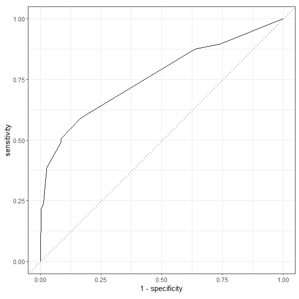
4.4. Area under the ROC
The ROC AUC tells us how good the model is at separating the 2 classes of the outcome.
# AUC ROC
roc_auc(df_preds, truth = Survived, .pred_Yes, event_level = "second")
## A tibble: 1 x 3
#  .metric .estimator .estimate
#  <chr>   <chr>          <dbl>
#1 roc_auc binary         0.760
Note that we set event_level = "second" since the default behavior of the function roc_auc() is to consider the first class of the variable Survived as the event. But since the classes (Yes/No) will be considered alphabetically (No before Yes), in this case, we need to set the second level (Yes) as the event.
roc_curve(df_preds, truth = Survived, .pred_Yes, event_level = "second") |>
  autoplot()
Output: