The objective of this article is to prove that getting a p-value below the threshold of 0.05 is not that hard, and that a statistically significant result proves nothing by itself.
Study results should always be interpreted in the context of:
- The study design
- The effect size
- The size of the sample
- The results of previous studies
Here is a list of the top 7 tricks that can be used to get statistically significant p-values:
- Using multiple testing
- Increasing the sample size
- Handling missing values in the way that benefits you the most
- Adding/removing other variables from the model
- Trying different statistical tests
- Categorizing numeric variables
- Grouping similar variables
Below we will discuss each of these points in details.
But first, note that none of these methods is inherently wrong, still they can be deceptive in some cases especially when combined with HARKing (Hypothesizing After the Results are Known) — i.e. when the study hypothesis is guided by the data itself that will be used to prove it.
In other words, to HARK is to:
- Find a solution,
- Then assign it to a problem,
- Finally, present your findings as if you thought of the problem first and then came up with the solution.
So let’s take a closer look at these “tricks” to see how each of them works:
1. Using multiple testing
If you torture the data long enough, it will confess to anything.
Ronald Coase
Multiple testing is based on the idea that:
“If we test the relationship between 2 non-related variables, the probability of getting a p-value < 0.05 is 5%”.
This statement can be easily proven with this simple simulation:
The simulation consists of repeating the following steps:
- Create 2 NON-related, normally distributed, random variables
- Compare them using a t-test
- Record the p-value
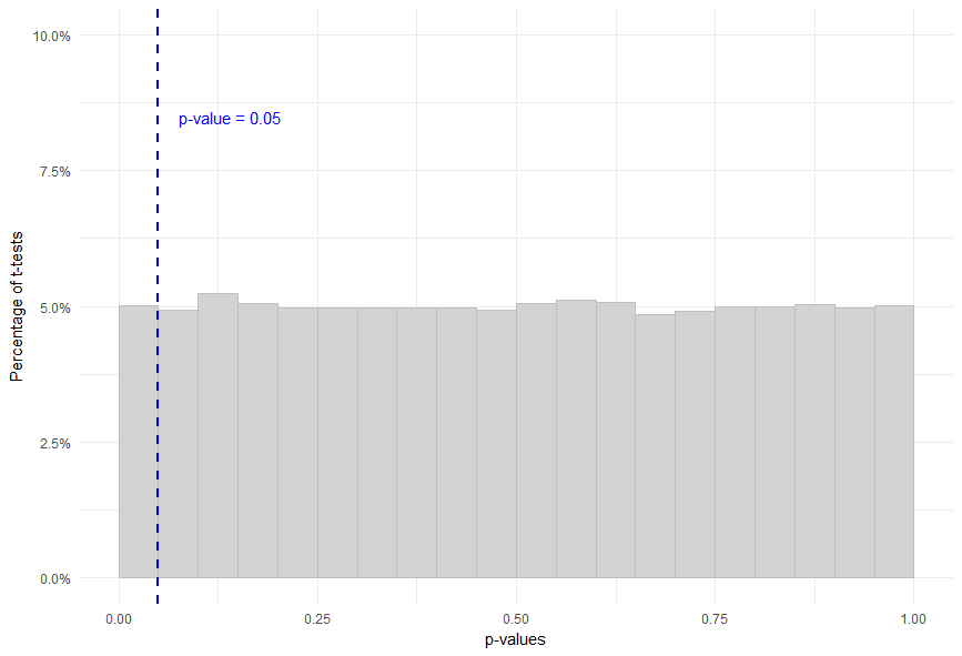
The histogram below shows the distribution of these p-values:

The first thing to notice is that the distribution is uniform.
This means that:
Prob(p-value < 0.05) = Prob(0.05 < p-value < 0.1) = Prob(0.1 < p-value < 0.15) = … = 5%
As you can see, even though the 2 variables are not related in any way, there is a 5% chance of getting a statistically significant result!
So we can take advantage of the results of our simulation and keep testing multiple predictor variables non-related to the outcome until we get a p < 0.05.
Each test we run will have a 5% probability of showing a statistically significant result.
This means that if we test 20 variables, on average, 1 will have a statistically significant effect, and this is due to chance only!
The next step is to search the literature for a relationship between the predictor that was found to have a p < 0.05 and the outcome, and tell our story backwards — That we first did a literature review, then tested the predictor and got a statistically significant result.
Be doubtful of statistically significant results from studies that were not replicated, especially if these studies were not pre-registered (which requires the researchers to state their hypotheses before data collection and analysis, therefore eliminating the problem of multiple testing).
2. Increasing the sample size
As discussed above, when there is no effect, the probability of getting a p < 0.05 is 5% — This is the probability of having a false positive result.
However, when there is a true effect, the probability of getting a p < 0.05 is… well it depends on the statistical power of your study.
The more statistical power you have, the more likely you’re going to detect an effect (assuming there is one).
One way of improving the statistical power is to increase the size of your sample. (for more information about statistical power, see Statistical Power: What it is and Why it Matters)
So once you know that a predictor has some effect on the outcome, it is not hard to get a p < 0.05 if you can increase the size of your sample.
Now you may be wondering: Where’s the trick if the predictor actually has a true effect on the outcome?
To which the answer is:
- You only need a VERY SMALL effect for this to work.
- It would be highly unlikely that the predictor under consideration has exactly zero effect on the outcome, or else it would not be taken seriously in the first place.
For instance, if a variable X has a very small, practically non-significant effect on the outcome Y, you can still get a statistically significant result just by working with a large enough sample.
To prove this point, I ran another simulation to study 2 cases:
First the case where the coefficient of X, the independent variable, is 0.1 (i.e. the case where the true relationship between X and Y is represented by the equation: Y = 0.1*X + ε).
Here’s a description of this simulation:
For different sample sizes repeat the following steps:
- Create a random, normally distributed, variable X
- Create Y, such that Y = 0.1*X + ε
- Regress Y onto X (i.e. run a linear regression)
- Check if the p-value for the coefficient of X is < 0.05
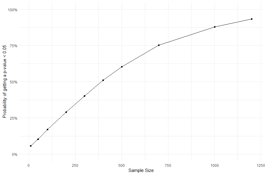
Here’s a graph that represents the probability of getting a statistically significant result versus the size of the sample:

You can see that when we increase the sample size, the probability of getting a statistically significant result increases.
With a sample size of 1200, we have almost a 100% chance of getting a p < 0.05.
Now let’s rerun the simulation with a smaller coefficient: 0.01 (i.e. with: Y = 0.01*X + ε).
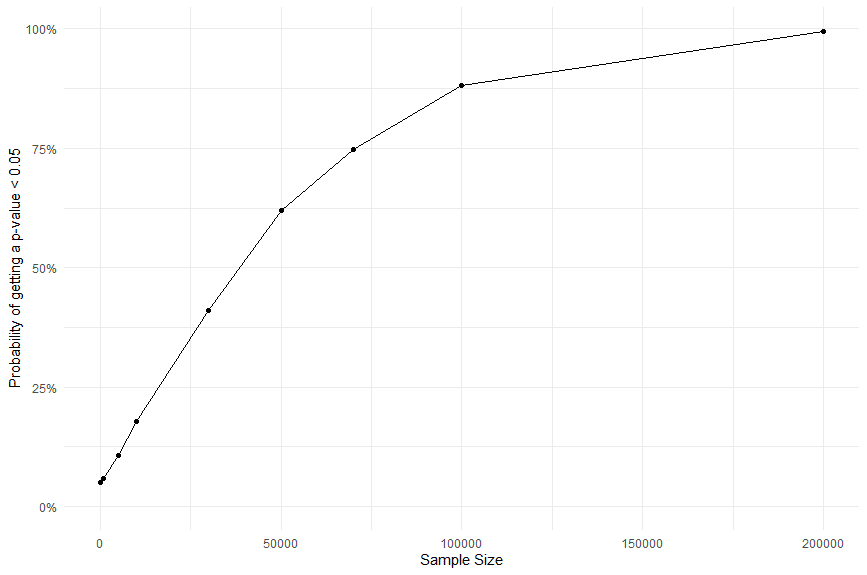
And here’s the corresponding graph:

Can you spot the difference?
Here we will need a larger sample size (~200,000) to guarantee a p < 0.05.
Despite having a very small, clinically insignificant effect of an independent variable on an outcome, we can still get a statistically significant result by increasing the sample size.
3. Handling missing values in the way that benefits you the most
Few objective rules exist for handling missing data. In most cases, the data analyst him/herself decides how to handle the situation based on several factors (such as the importance of the variable that has missing values, the percentage of missing values, etc.).
So we can argue that there is some room for subjectivity in handling missing values that will allow us to control the study outcome.
A simple example would be a situation where by imputing missing values we increase the sample size enough to get the required statistical power to reject the null hypothesis (get a p < 0.05).
In this case, we can either choose to impute missing values and get a statistically significant result, or to delete them and get a p-value > 0.05.
This trick works because the way we choose to handle missing values is directly related to the size of the sample that we are working with:

P-values may also be sensitive to the method of imputation (replacing missing values with the variable’s mean, median or mode, using a regression or other more complex imputation models).
Study pre-registration is key as it requires researchers to state how they will handle missing values even before collecting data. Another solution is to report results of the statistical analysis run both before and after imputation and the reader is left to compare results and judge. Otherwise you should question the researcher’s choice of the method used to handle missing data, whether or not it was based on solid reasoning/guidelines.
4. Adding/removing other variables from the model
When studying the relationship between a predictor Xi and an outcome Y, adding and removing other variables from the model may affect the coefficient of Xi and the p-value associated with it.
Sometimes the causal structure between predictor variables is not clear, which leaves room for a little bit of subjectivity in deciding which variables to include/exclude from the model:
- Excluding a covariate (another variable that affects the outcome) that is correlated with Xi will inflate the regression coefficient and reduce the p-value of Xi.
- Excluding a confounding variable will have the same effect.
- Including (in a linear regression model) a covariate correlated to Xi, or a confounding variable, that are non-linearly related to the outcome will make the coefficient and p-value of Xi appear more significant than they really are.
When selecting variables for a regression model, one of the most important things the researcher should take into consideration is the causal relationships between them. Also all technical aspects must be considered and reported, especially the assumption of linearity between independent and dependent variables in the case of linear regression.
5. Trying different statistical tests
Choosing between a parametric and a non-parametric statistical test depends on the distribution of your data.
In some cases, deciding whether a variable is normally distributed or not is a subjective exercise, thus opening the possibility for gaming the system.
Another example is the large array of post-hoc tests available for correction after running a one-way ANOVA. As some of these tests are more conservative than others, we can choose the correction that is in line with our purposes to either support or challenge a hypothesis.
Again pre-registration of studies plays a big role in preventing this kind of data dredging.
6. Categorizing numeric variables
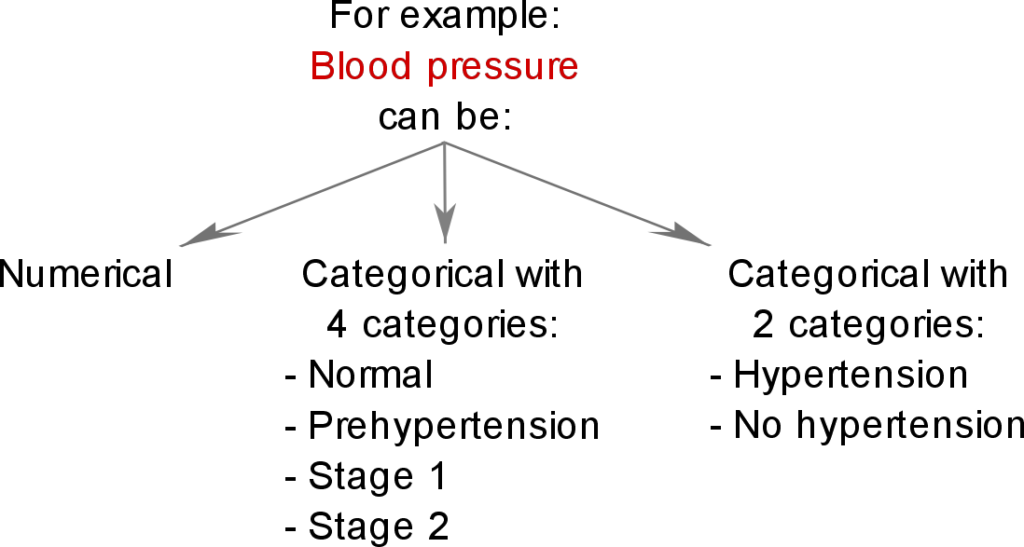
Transforming a continuous variable into a categorical one is generally not advisable as it risks losing information.
However, in some cases, it offers a way of dealing with a non-linear relationship between independent and dependent variables when running linear regression.
Several decisions must be made here:
- Whether the numeric or categorical version of a given variable should be used
- The number of categories
- The thresholds or range for each category

Trying different combination of options can yield different effect sizes and p-values.
In some cases, for instance when studying alcohol consumption, it may be valid to use a categorical version of age: under-legal-age and over-legal-age. However, this should be specified before running any statistical test on the data.
7. Grouping similar variables
Let’s consider the following example:
Assume that a given drug has the side effect of increasing the risk of stroke, however, it does not affect the risk of heart attacks and arrhythmia.
One evil trick we can do is to combine all these diseases into 1 variable — cardiovascular disease.

And then test the effect of the drug on the new variable: cardiovascular disease.
This can dilute the effect of the drug and thus lead us to conclude that it does not increase the risk of cardiovascular diseases in general.
This effect can go both ways.
If the effect is large enough between an independent variable and an outcome, combining the independent variable with others will increase the chance of getting a p < 0.05 for the combined variables.
I hope by now you’re convinced of the power of pre-registration. Also, sharing data after publication (if legally possible) is very important for others to rerun your analysis and support your conclusions.
Further reading
- Which Variables to Include in a Regression Model
- Why and When to Include Interactions in a Regression Model
- Standardize vs Unstandardized Regression Coefficients
- Correlation vs Collinearity vs Multicollinearity
- Statistical Power: What it is and Why it Matters
- Statistical Software Popularity in 40,582 Research Papers