The conditional distribution of a variable, for example heights, is the distribution of heights given the value of another variable, for example gender. Plotting the conditional distribution of heights given gender is a way of visualizing the relationship between the 2 variables.
The marginal distribution of heights is the distribution of heights for everybody, independent of gender. Plotting the marginal distribution of heights is a way of describing the probability of occurrence of each value of the variable.
If heights was a numerical variable
The density plot below represents the marginal and conditional distributions of heights:
- The dashed curve is the marginal distribution of heights — the distribution of everybody’s heights regardless of their gender.
- The pink and blue curves are the conditional distributions:
- The pink curve is the distribution of heights given that the gender is female.
- The blue curve is the distribution of heights given that the gender is male.
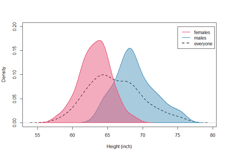
The conditional distribution of males is shifted to the right which means that, on average, males are taller than females. The marginal distribution is bimodal which reflects the fact that it is the combination of the 2 conditional distributions.
If heights was a categorical variable
Now consider the case where heights is a binary categorical variable that can take on 2 values: “Tall” or “Normal/Short”.
The following bar plot represents the marginal distribution of heights (regardless of gender):
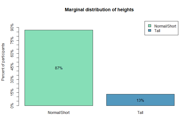
The bar plot shows that 13% of all participants are tall, and 87% are either normal or short.
The following stacked bar plot represents the distribution of heights conditional on gender:
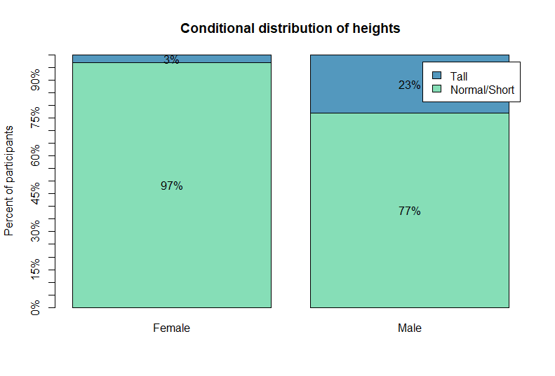
Given that the person is female, then the probability of being tall is only 3%; And given that the person is male, this probability is 23%.
The conditional distribution of a categorical variable can also be represented in a table:
| Female | Male | |
|---|---|---|
| Normal/Short | 97% | 77% |
| Tall | 3% | 23% |
R code
Here’s the R code that generated these plots:
## marginal and conditional distributions of a numerical variable
#################################################################

set.seed(1)
# sample female heights from a normal distribution
# with mean = 63 and std = 2.5
female.heights = rnorm(n = 100, mean = 63, sd = 2.5)

# sample male heights from a normal distribution
# with mean = 69 and std = 3
male.heights = rnorm(n = 100, mean = 69, sd = 3)

# combine female and male data
all.heights = c(male.heights, female.heights)


plot(density(all.heights), # plot density of all heights
     lwd = 2, # line thickness
     ylim = c(0, 0.2), # y-axis limits
     lty = 2, # dashed line
     main = '', # remove title
     xlab = 'Height (inch)') # x-axis label

polygon(density(male.heights), # plot density of male heights
        col = rgb(0.325, 0.596, 0.745, alpha = 0.5), # fill color
        border = '#5398BE', # line color
        lwd = 2) # line thickness

polygon(density(female.heights), # plot density of female heights
        col = rgb(0.906, 0.353, 0.486, alpha = 0.5), # fill color
        border = '#E75A7C', # line color
        lwd = 2) # line width

legend(x = 75, y = 0.2, # coordinates of the legend
       legend = c("females", "males", "everyone"),
       col = c("#E75A7C", "#5398BE", "black"),
       lty = c(1, 1, 2),
       lwd = 2)


## marginal and conditional distributions of a categorical variable
###################################################################

dat = data.frame(gender = c(rep('Female', 100), rep('Male', 100)),
                heights = c(female.heights, male.heights))

# males above 71 inches are tall
dat$isTall[dat$gender == 'Male' & dat$heights >= 71] = 'Tall'
# males below 71 inches are normal/short
dat$isTall[dat$gender == 'Male' & dat$heights < 71] = 'Normal/Short'

# females above 67 inches are tall
dat$isTall[dat$gender == 'Female' & dat$heights >= 67] = 'Tall'
# females below 67 inches are normal/short
dat$isTall[dat$gender == 'Female' & dat$heights < 67] = 'Normal/Short'


# marginal distribution of isTall
library(scales) # to show percentages on the y-axis
x = barplot(prop.table(table(dat$isTall)),
            col = rep(c('#86DEB7', '#5398BE')),
            legend = TRUE,
            yaxt = 'n', # remove y-axis
            ylab = 'Percent of participants',
            ylim = c(0, 1),
            main = 'Marginal distribution of heights')
# creating a y-axis with percentages
yticks = seq(0, 0.9, by = 0.05)
axis(2, at = yticks, lab = percent(yticks))
# showing the values of each category
y = prop.table(table(dat$isTall))
text(x[1], y[1]/2, labels = paste0(as.character(y[1]*100), '%')) # placing Normal/short values
text(x[2], y[2]/2, labels = paste0(as.character(y[2]*100), '%')) # placing Tall values


# distribution of isTall conditional on gender
library(scales) # to show percentages on the y-axis
x = barplot(prop.table(table(dat$isTall, dat$gender), 2),
            col = rep(c('#86DEB7', '#5398BE')),
            legend = TRUE,
            yaxt = 'n', # remove y-axis
            ylab = 'Percent of participants',
            ylim = c(0, 1),
            main = 'Conditional distribution of heights')
# creating a y-axis with percentages
yticks = seq(0, 1, by = 0.05)
axis(2, at = yticks, lab = percent(yticks))
# showing the values of each category
y = prop.table(table(dat$isTall, dat$gender), 2)
text(x, y[1,]/2, labels = paste0(as.character(y[1,]*100), '%')) # placing Normal/short values
text(x, y[1,] + y[2,]/2, labels = paste0(as.character(y[2,]*100), '%')) # placing Tall values
For a tutorial on how to use the functions table() and prop.table(), see: How to Describe/Summarize Categorical Data in R (Example).