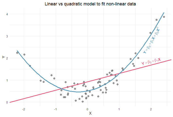
Linear regression assumes that the relationship between the predictor X and the outcome Y is linear.
If this assumption is not met, linear regression will be a poor fit to the data (as shown in the figure below). In this case, adding a quadratic term to the regression equation may help model the relationship between X and Y.
The equation becomes:
\(Y = β_0 + β_1 X + β_2 X^2\)
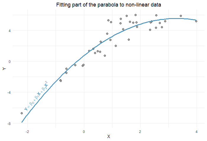
Note that the quadratic model does not require the data to be U-shaped. Other curves can also be fitted using just a part of the parabola, as we see below:
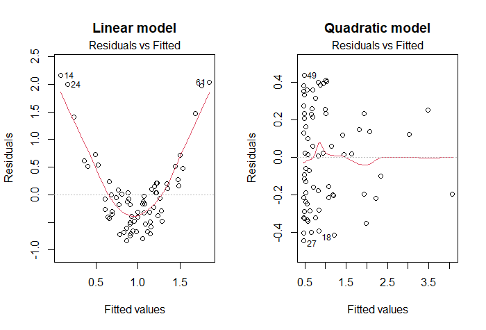
When to add a quadratic term?
Start by fitting a linear regression model to the data (\(Y = β_0 + β_1 X\)), and plot the residuals versus the fitted values. If this plot shows some pattern (for example, the U-shaped pattern in the left side of the figure below), try adding a quadratic term to the model (\(Y = β_0 + β_1 X + β_2 X^2\)). If the pattern disappears (see right side of the figure below), then conclude that the quadratic model is a better fit to the data.
Besides looking at the residuals vs fitted values, we can also assess the fit of the quadratic model by comparing the adjusted R-squared between the linear and the quadratic model, or by checking the statistical significance of the quadratic term’s coefficient (i.e. if p < 0.05).
Other options to correct a non-linear relationship between X and Y is to use a logarithmic or a square root transformation of X. (For more information, I recommend an article I wrote on using variable transformations to improve your regression model).
How to interpret a model with a quadratic term?
In a quadratic model, the variable X is associated with 2 coefficients β1 and β2 (\(Y = β_0 + β_1 X + β_2 X^2\)), so its effect will no longer have a straightforward interpretation.
But before going into the details of this interpretation, let’s first review how to interpret the effect of X on Y in a linear model \(Y = β_0 + β_1 X\). In this case:
β1 is the change in Y associated with a 1 unit change in X.
Mathematically, β1 is the derivative of Y with respect to X (denoted \(\frac{dY}{dX}\)), that tells us how much Y changes with a 1 unit change in X.
So, for a linear model: \(Y = β_0 + β_1 X\) and \(\frac{dY}{dX} = β_1\).
But, for a quadratic model: \(Y = β_0 + β_1 X + β_2 X^2\) and \(\frac{dY}{dX} = β_1 + 2 β_2 X\).
And the interpretation becomes:
(β1 + 2 β2 X) is the change in Y associated with a 1 unit change in X.
Unlike the linear model, the change in Y now depends on the value of X. In other words, the effect of X is not constant anymore.
So, to interpret the effect of X on Y, we need to specify the value of X.
Let’s look at an example.
Example: Interpreting the effect of BMI on blood pressure
Here’s a plot of the relationship between BMI and systolic blood pressure (SBP):
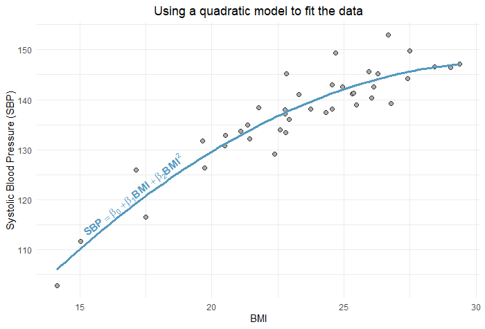
And here’s the output of the quadratic model used to fit the data:
| Variable | Coefficient | Standard error | p-value |
|---|---|---|---|
| (Intercept) | 8.57 | 17.51 | 0.628 |
| BMI | 8.90 | 1.59 | < 0.001 |
| BMI2 | -0.14 | 0.04 | < 0.001 |
Using this table, we can write the regression equation:
\(SBP = 8.57 + 8.9 BMI – 0.14 BMI^2\)
And calculate the derivative \(\frac{dSBP}{dBMI}\) (i.e. the change in systolic blood pressure for a 1 unit change in BMI):
\(\frac{dSBP}{dBMI} = 8.9 – 0.28 BMI\).
Now, we can interpret the effect of BMI on systolic blood pressure for different values of BMI:
1. For an underweight person with a BMI of 15:
\(\frac{dSBP}{dBMI} = 8.9 – 0.28 × 15 = 4.7\).
Therefore:
For underweight people with a BMI around 15, 4.7 is the change in systolic blood pressure associated with a 1 unit change in BMI.
In other words:
4.7 is the expected difference in systolic blood pressure when comparing 2 groups of underweight people, with a BMI around 15, who differ by 1 unit in BMI.
2. For an overweight person with a BMI of 28:
\(\frac{dSBP}{dBMI} = 8.9 – 0.28 × 28 = 1.06\).
The first thing to notice is that systolic blood pressure does not change as much with BMI for overweight people compared to underweight people. In other words, the higher the BMI the weaker its association with systolic blood pressure.
We can interpret the effect of 1.06 as follows:
For overweight people with a BMI around 28, 1.06 is the change in systolic blood pressure associated with a 1 unit change in BMI.
In other words:
1.06 is the expected difference in systolic blood pressure when comparing 2 groups of overweight people, with a BMI around 28, who differ by 1 unit in BMI.
References
- Huntington-Klein N. The Effect. 1st edition. Routledge; 2022.
- James G, Witten D, Hastie T, Tibshirani R. An Introduction to Statistical Learning: With Applications in R. 2nd edition. Springer; 2021.