The residual standard deviation (or residual standard error) is a measure used to assess how well a linear regression model fits the data. (The other measure to assess this goodness of fit is R2).
But before we discuss the residual standard deviation, let’s try to assess the goodness of fit graphically.
Consider the following linear regression model:
Y = β0 + β1X + ε
Plotted below are examples of 2 of these regression lines modeling 2 different datasets:
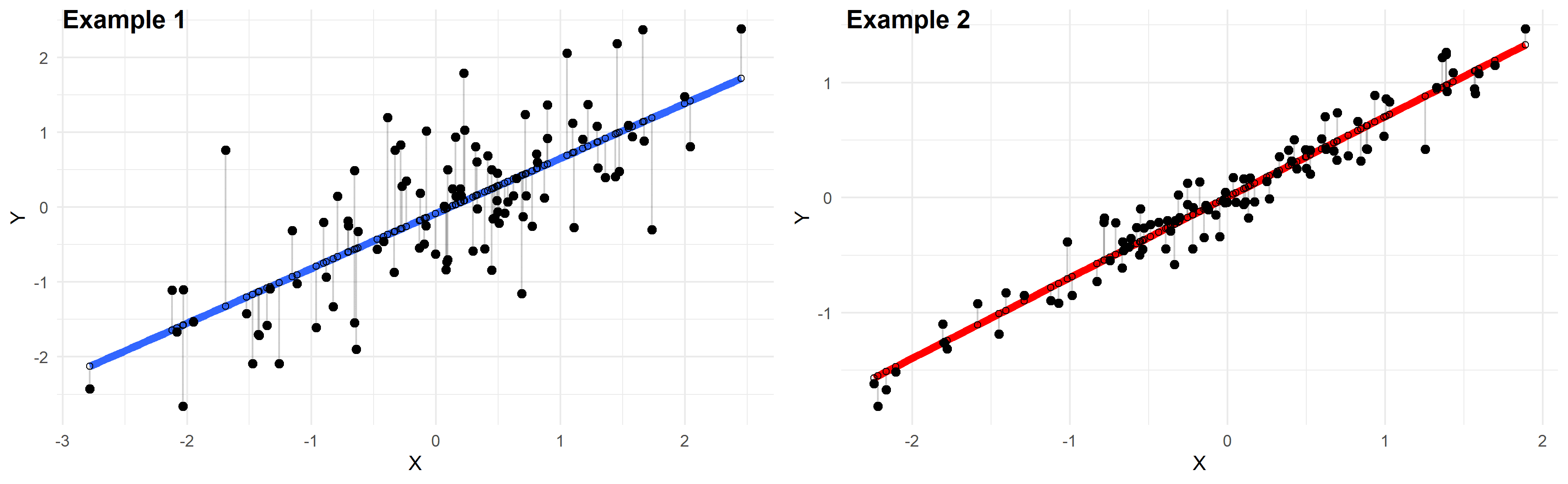
Just by looking at these plots we can say that the linear regression model in “example 2” fits the data better than that of “example 1”.
This is because in “example 2” the points are closer to the regression line. Therefore, using a linear regression model to approximate the true values of these points will yield smaller errors than “example 1”.
In the plots above, the gray vertical lines represent the error terms — the difference between the model and the true value of Y.
Mathematically, the error of the ith point on the x-axis is given by the equation: (Yi – Ŷi), which is the difference between the true value of Y (Yi) and the value predicted by the linear model (Ŷi) — this difference determines the length of the gray vertical lines in the plots above.
Now that we developed a basic intuition, next we will try to come up with a statistic that quantifies this goodness of fit.
Residual standard deviation vs residual standard error vs RMSE
The simplest way to quantify how far the data points are from the regression line, is to calculate the average distance from this line:
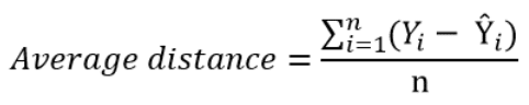
Where n is the sample size.
But, because some of the distances are positive and some are negative (certain points are above the regression line and others are below it), these distances will cancel each other out — meaning that the average distance will be biased low.
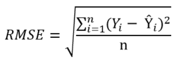
In order to remedy this situation, one solution is to take the square of this distance (which will always be a positive number), then calculate the sum of these squared distances for all data points and finally take the square root of this sum to obtain the Root Mean Square Error (RMSE):
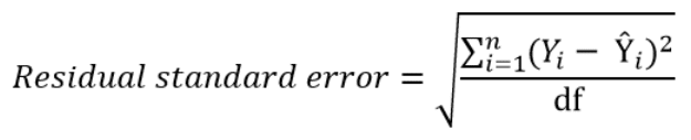
We can take this equation one step further:
Instead of dividing by the sample size n, we can divide by the degrees of freedom df to obtain an unbiased estimation of the standard deviation of the error term ε. (If you’re having trouble with this idea, I recommend these 4 videos from Khan Academy which provide a simple explanation mainly through simulations instead of math equations).
The quantity obtained is sometimes called the residual standard deviation (as referred to it in the textbook Data Analysis Using Regression and Multilevel Hierarchical Models by Andrew Gelman and Jennifer Hill). Other textbooks refer to it as the residual standard error (for example An Introduction to Statistical Learning by Gareth James, Daniela Witten, Trevor Hastie and Robert Tibshirani).
In the statistical programming language R, calling the function summary on the linear model will calculate it automatically.
The degrees of freedom df are the sample size minus the number of parameters we’re trying to estimate.
For example, if we’re estimating 2 parameters β0 and β1 as in:
Y = β0 + β1X + ε
Then, df = n – 2
If we’re estimating 3 parameters, as in:
Y = β0 + β1X1 + β2X2 + ε
Then, df = n – 3
And so on…
Now that we have a statistic that measures the goodness of fit of a linear model, next we will discuss how to interpret it in practice.
How to interpret the residual standard deviation/error
Simply put, the residual standard deviation is the average amount that the real values of Y differ from the predictions provided by the regression line.
We can divide this quantity by the mean of Y to obtain the average deviation in percent (which is useful because it will be independent of the units of measure of Y).
Here’s an example:
Suppose we regressed systolic blood pressure (SBP) onto body mass index (BMI) — which is a fancy way of saying that we ran the following linear regression model:
SBP = β0 + β1×BMI + ε
After running the model we found that:
- β0 = 100
- β1 = 1
- And the residual standard error is 12 mmHg
So we can say that the BMI accurately predicts systolic blood pressure with about 12 mmHg error on average.
More precisely, we can say that 68% of the predicted SBP values will be within ∓ 12 mmHg of the real values.
Why 68%?
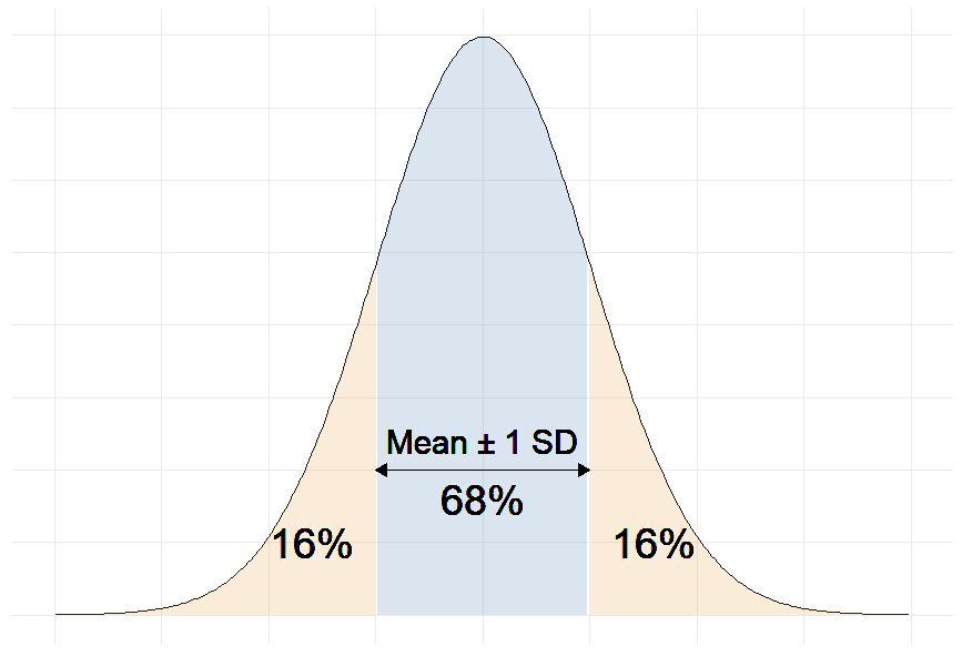
Remember that in linear regression, the error terms are Normally distributed.
And one of the properties of the Normal distribution is that 68% of the data sits around 1 standard deviation from the average (See figure below).
Therefore, 68% of the errors will be between ∓ 1 × residual standard deviation.
For example, our linear regression equation predicts that a person with a BMI of 20 will have an SBP of:
SBP = β0 + β1×BMI = 100 + 1 × 20 = 120 mmHg.
With a residual error of 12 mmHg, this person has a 68% chance of having his true SBP between 108 and 132 mmHg.
Moreover, if the mean of SBP in our sample is 130 mmHg for example, then:
12 mmHg ÷ 130 mmHg = 9.2%
So we can also say that the BMI accurately predicts systolic blood pressure with a percentage error of 9.2%.
The question remains: Is 9.2% a good percent error value? More generally, what is a good value for the residual standard deviation?
The answer is that there is no universally acceptable threshold for the residual standard deviation. This should be decided based on your experience in the domain.
In general, the smaller the residual standard deviation/error, the better the model fits the data. And if the value is deemed unacceptably large, consider using a model other than linear regression.