A square root transformation can be useful for:
- Normalizing a skewed distribution
- Transforming a non-linear relationship between 2 variables into a linear one
- Reducing heteroscedasticity of the residuals in linear regression
- Focusing on visualizing certain parts of your data
Below we will discuss each of these points in details.
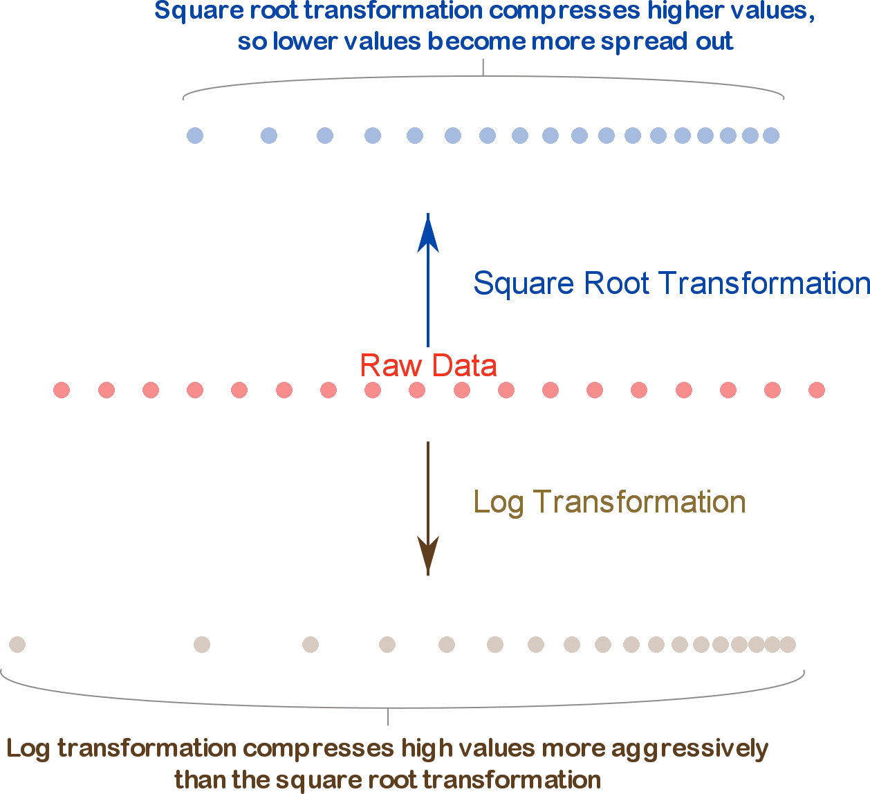
When you apply a square root transformation to a variable, high values get compressed and low values become more spread out. Log transformation does the same thing but more aggressively.
Note: Be careful when using a square root transformation on variables that have negative values or you will end up with a lot of missing values. The problem is that these will NOT be missing at random, and therefore will bias your analysis.
1. Square root transformation for normalizing a skewed distribution
When you want to use a parametric hypothesis test (especially if you have a small sample size), you need to ensure that the variable under study is normally distributed.
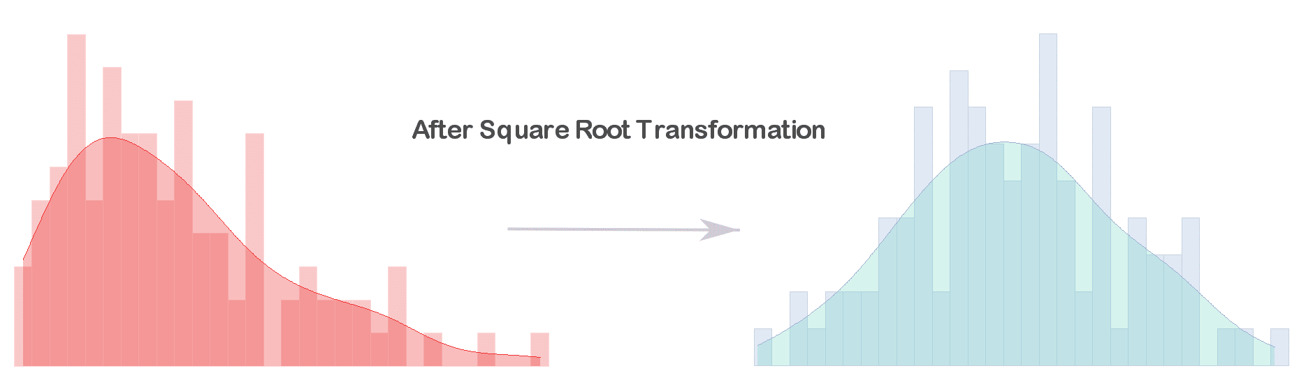
If your variable has a right skew, you can try a square root transformation in order to normalize it.
Examples of variables with a right skew include: income distribution, age, height and weight.
Another situation where you might need a square root transformation is when the distribution of the residuals (a.k.a. error terms) of a regression model is not normal. In this case, using a square root transformation on the outcome variable (dependent variable) may yield normally distributed residuals.
The regression model obtained may become more “correct” statistically, but it will certainly become less interpretable.
Note that when using a regression model for understanding the relationship between the independent variables and the outcome, the assumption of normality (of the residuals) is not that important. On the other hand, if you’re using linear regression for prediction purposes (i.e. creating a model to predict the outcome given the independent variables) then you should make sure that the residuals are normally distributed. [Source: Data Analysis Using Regression and Multilevel Hierarchical Models]
Personally, I never worry about normality of the residuals since I don’t use linear regression for prediction purposes as other non-linear models provide better out-of-sample accuracy. (For prediction, more often than not, gradient boosted trees will outperform all other models).
The square root transformation will not fix all skewed variables. Variables with a left skew, for instance, will become worst after a square root transformation. As discussed above, this is a consequence of compressing high values and stretching out the ones on the lower end.
In order to normalize left skewed distributions, you can try a quadratic, cube or exponential transformation.
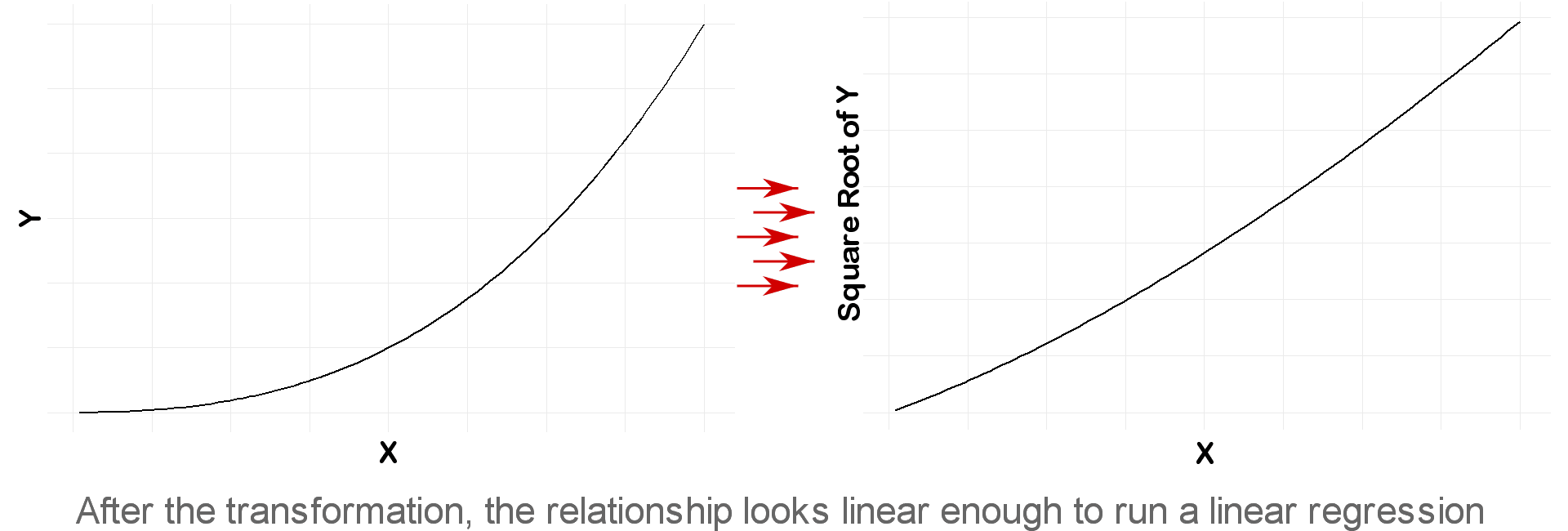
2. Square root transformation for transforming a non-linear relationship into a linear one
When running a linear regression, the most important assumption is that the dependent and independent variable have a linear relationship.
One solution to fix a non-linear relationship between X and Y, is to try a log or square root transformation.
However, as discussed in the previous section, the model’s coefficients once again will become less interpretable, but at least they will be statistically correct.
Here’s an example where interpreting the coefficient of each independent variable is not that important:
Suppose your objective is to compare the importance of various factors in predicting a certain outcome, and you decided to do so using a linear regression model. In this case, using a square root transformation of Y will affect the interpretation of each coefficient alone, but will not interfere with your objective.
3. Square root transformation for reducing heteroscedasticity
Another assumption of linear regression is that the residuals should have equal variance (often referred to as homoscedasticity of the residuals).
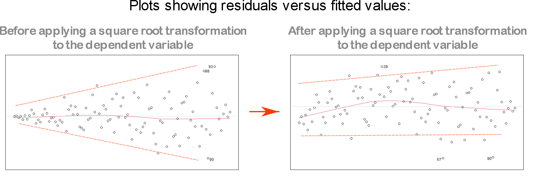
When the plot of residuals versus fitted values shows a funnel shape (as seen in the left-hand plot of the figure below), it is considered a sign of non-equal variance of the residuals (i.e. a sign of heteroscedasticity).
To address this issue, one solution is to use a logarithmic or square root transformation on the outcome Y:
For more information on how to deal with violations of linear regression assumptions, I recommend: 5 Variable Transformations to Improve Your Regression Model.
4. Square root transformation for clearer visualizations
Some variables will inherently have very low and very high values when measured at different times. This will make them a little bit harder to visualize in a single plot.
An example of such variable is the blood CRP (C-Reactive Protein), which is a marker of inflammation in the body. Its normal range is less than 6 mg/L. But in case of bacterial infection, it could be as high as 10 times the normal value (so > 60 mg/L).
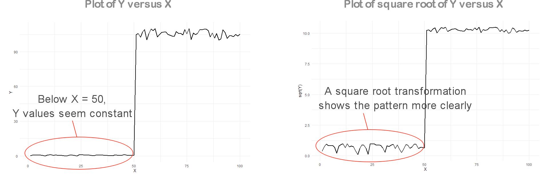
Below is an example of a variable Y plotted against X. As you may have noticed in the left-hand plot, low values of Y cannot be distinguished from one another and appear to be constant below X = 50.
In this case, a square root transformation may help visualize the pattern of these lower values of Y (right-hand plot).
Be careful, however, to clearly mention and defend any transformation or change you make to your data before plotting them. Otherwise, you may be accused of misleading your readers.