Understand Linear Regression Assumptions

The 4 assumptions of linear regression in order of importance are:

1. Linearity
2. Independence of errors
3. Constant variance of errors
4. Normality of errors

1. Linearity

1.1. Explanation

The relationship between each predictor X_i and the outcome Y should be linear.

1.2. How to check the linearity assumption

Instead of checking the relationship between each predictor X_i and the outcome Y in a multivariable model, we can plot the residuals versus the fitted values. The plot should show no pattern:

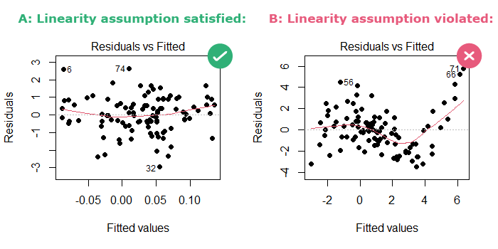
In the figure above, we can focus on the LOESS red line that smoothly fits the data:

• In part A: The LOESS line looks like “a child’s freehand drawing of a straight line” [Cohen et al. 2002], so the linearity assumption is satisfied.
• In part B: the LOESS line is curved, so the linearity assumption is violated.

1.3. What happens when the linearity assumption is violated

When this assumption is violated, we may get:

• Biased regression coefficients
• Biased standard errors
• Biased p-values
• Biased R²

So linearity is the most important linear regression assumption since its violation biases all the model’s output.

1.4. How to deal with non-linearity

When the linearity assumption is violated, try:

• Adding a quadratic term to the model: Y = X₁ + X₁² + X₂ + X₂²
• Transforming the predictor X (log, square root): Y = log(X₁) + log(X₂)
• Adding an interaction term (since non-linearity can be due to an interaction between predictors): Y = X₁ + X₂ + X₁×X₂
• Categorizing the predictor X (when X is a numeric variable)

How to check if your solution works:

• If you added a quadratic or an interaction term: you can use ANOVA to compare the model with the quadratic or interaction term to one without them.
• If you used a log or square root transformed predictor: an increase in the adjusted-R² for the new model would be a sign of a better fit.

Here’s a tutorial on how to implement these fixes in R.

2. Independence of errors

2.1. Explanation

Independent/uncorrelated error terms are obtained if each observation is drawn randomly from the population.

2.2. How to check the independence of errors

This assumption is violated in time series, spatial, and multilevel settings. So check the study design and the data collection process.

For example, errors can be correlated when we are dealing with multiple measurements made on the same participants, or when cluster sampling is used.

2.3. What happens when errors are not independent

When the independence of errors assumption is violated, we may get:

• Biased standard errors (smaller standard errors and confidence intervals)
• Biased p-values (smaller p-values)

So independence of errors is useful to assess whether the confidence intervals and p-values can be trusted.

2.4. How to deal with correlated errors

The fix depends on how the errors are correlated. You should use a data analysis method that is appropriate for your study design (for example, an ARIMA model can be used for time series data, and a multilevel model for nested data).

3. Constant variance of errors

3.1. Explanation

The dispersion of the data around the regression line should be constant.

3.2. How to check the constant variance of errors

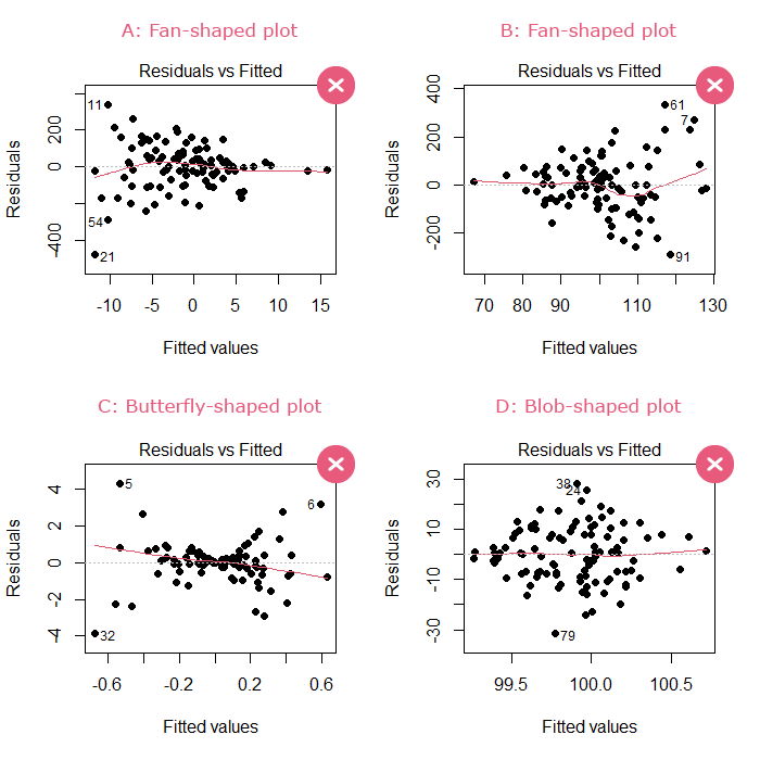
The plot of the residuals versus the fitted values should show no discernible shape. A fan, butterfly, or blob shape are signs of violation of this assumption:

What if the predictor X is a categorical variable?

In this case, calculate the variance of the residuals for each subgroup of X. The constant variance assumption will be violated if the variance of the residuals:

• Changes by a factor of 2 or more between subgroups that differ in size by a factor of 2 or more.
• Changes by a factor of 3 or more between subgroups that differ in size by a factor of less than 2.

[source: Huntington-Klein, 2022]

3.3. What happens when errors do not have constant variance

When the assumption of constant variance of errors is violated, we may get:

• Biased standard errors
• Biased p-values

Note that this assumption is less important for estimating the relationship between a predictor X and an outcome Y. It is more important for predictive modeling, when the objective of using linear regression is to predict Y given X.

3.4. How to deal with non-constant error variance

When the assumption of constant variance of errors is violated, try:

• Transforming the outcome Y (log, square root)
• Using weighted regression
• Calculating heteroscedasticity-robust standard errors
• Converting the outcome into a binary variable then using logistic regression (least favorable solution)

Here’s a tutorial on how to implement these fixes in R.

4. Normality of errors

4.1. Explanation

Error terms should be normally distributed.

4.2. How to check the normality of errors

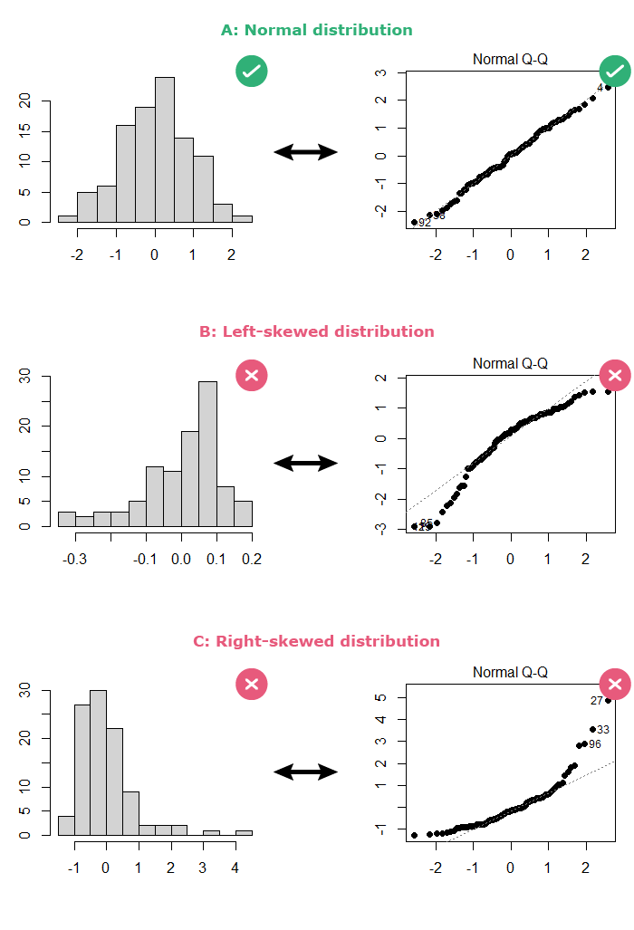
The normality of the errors can be checked in 2 ways:

1. By looking at a histogram of the residuals: the distribution should be bell-shaped.
2. By looking at a normal Q-Q plot of the residuals: The points should follow the diagonal straight line.

Here are some examples:

4.3. What happens when errors are not normally distributed

When the normality of errors assumption is violated, we may get:

• Biased standard errors
• Biased p-values

This is the least important of the linear regression assumptions since it should be taken into consideration only in 2 cases:

1. When working with a small sample size.
2. When using linear regression for prediction purposes, i.e. when calculating prediction intervals. Instead, when the objective is to estimate the relationship between a predictor X and an outcome Y, Gelman and colleagues do not even recommend checking the normality of the residuals.

4.4. How to deal with non-normal errors

When the normality of errors assumption is violated, try:

• Transforming the outcome Y (log, square root)
• Removing outliers (observations with Y values that are far from the regression line)
• Transforming the outcome into a binary variable then using logistic regression (least favorable solution)

Here’s a tutorial on how to implement these fixes in R.

References

• Keith TZ. Multiple Regression and Beyond: An Introduction to Multiple Regression and Structural Equation Modeling. 3rd edition. Routledge; 2019.
• Vittinghoff E, Glidden DV, Shiboski SC, McCulloch CE. Regression Methods in Biostatistics: Linear, Logistic, Survival, and Repeated Measures Models. 2nd ed. 2012 edition. Springer; 2011.
• Gelman A, Hill J, Vehtari A. Regression and Other Stories. 1st edition. Cambridge University Press; 2020.
• Cohen J, Cohen P, West SG, Aiken LS. Applied Multiple Regression/Correlation Analysis for the Behavioral Sciences, 3rd Edition. Third edition. Routledge; 2002.
• Huntington-Klein N. The Effect. 1st edition. Routledge; 2022.

Further reading

• How to Check Linear Regression Assumptions in R
• Which Variables Should You Include in a Regression Model?
• 5 Variable Transformations to Improve Your Regression Model
• How to Handle Missing Data in Practice: Guide for Beginners
• Interpret Linear Regression Coefficients