A mixed model (also called a mixed-effects model) is used when the observations (i.e. rows) in the data are not independent. This can occur, for example, when measurements are taken from the same individuals multiple times or when observations can be grouped into clusters, such as families, co-workers, etc.
In this tutorial, we will run and interpret a mixed model, using the “mammals sleep” dataset (msleep) available from the ggplot2 package (included in tidyverse), to explore the relationship between brain weight in kilograms (brainwt) and the amount of time spent awake (awake), taking into consideration the animal’s classification (order).
1. Loading the data
First, we select the variables of interest and remove observations with missing values:
library(tidyverse)

msleep <-
  msleep |>
  select(brainwt, order, awake) |>
  drop_na()

msleep
## A tibble: 56 × 3
#   brainwt order        awake
#     <dbl> <chr>        <dbl>
# 1 0.0155  Primates       7
# 2 0.00029 Soricomorpha   9.1
# 3 0.423   Artiodactyla  20
# 4 0.07    Carnivora     13.9
# 5 0.0982  Artiodactyla  21
# 6 0.115   Artiodactyla  18.7
# 7 0.0055  Rodentia      14.6
# 8 0.0064  Rodentia      11.5
# 9 0.001   Soricomorpha  13.7
#10 0.0066  Rodentia      15.7
## ℹ 46 more rows
## ℹ Use `print(n = ...)` to see more rows
2. Why an ordinary linear regression will not work in this case
In theory, studying the effect of brain weight on the amount of time spent awake, while taking into consideration the order of the animal can be done with the following linear regression model:
awake = β0 + β1 brainwt + β2 order + ε
In this model, the coefficient β1 will reflect the relationship between brain weight and time spent awake, while controlling for the animal’s order. Except that in this case, the variable order has 17 categories with most categories containing just a few observations:
msleep |> count(order)
## A tibble: 17 × 2
#   order               n
#   <chr>           <int>
# 1 Afrosoricida        1
# 2 Artiodactyla        5
# 3 Carnivora           7
# 4 Chiroptera          2
# 5 Cingulata           2
# 6 Didelphimorphia     1
# 7 Diprotodontia       1
# 8 Erinaceomorpha      2
# 9 Hyracoidea          3
#10 Lagomorpha          1
#11 Monotremata         1
#12 Perissodactyla      3
#13 Primates            9
#14 Proboscidea         2
#15 Rodentia           10
#16 Scandentia          1
#17 Soricomorpha        5
A simple solution would be to remove order from the model. But then we would miss out on correlations inside each order that may not be detectable in the overall data. In this case, a mixed model can help us take into account the animal’s order.
3. Considerations before running a mixed model
Before we run the mixed model, let’s visualize the relationship between brain weight and hours spent awake:
msleep |>
  ggplot(aes(x = brainwt, y = awake)) +
  geom_point()
Output:
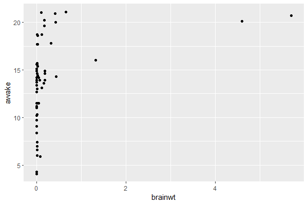
Most animals have a small brain weight, so let’s take the log of brain weight and visualize this relationship for different animal orders:
msleep |>
  ggplot(aes(x = brainwt, y = awake)) +
  geom_point(aes(color = order)) +
  geom_smooth(aes(color = order), se = FALSE, method = "lm") +
  geom_smooth(se = FALSE, method = "lm", color = "black") +
  scale_x_log10()
Output:
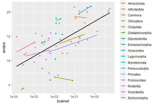
The black line shows the relationship between brain weight and hours awake for all animals in the sample, and the colored lines represent this same relationship inside each animal order.
Looking at this graph, we will suppose that these regression lines have (almost) the same slopes but different intercepts, so we will use a mixed model with a random intercept. In other words, we are assuming that order only changes the intercept of the regression line but does not affect its steepness.
4. Running a mixed model
To add a random intercept according to the animal order, we use the lmer() function instead of lm() and add the term (1|order) to the formula as follows:
(Note that for a categorical outcome, we use the same syntax but with a glmer() function instead of glm())
# remember that we decided to use log(brainwt), see the plot above
model <- lmer(awake ~ log(brainwt) + (1|order), data = msleep)

summary(model)
#Linear mixed model fit by REML ['lmerMod']
#Formula: awake ~ log(brainwt) + (1 | order)
#   Data: msleep
#
#REML criterion at convergence: 279.4
#
#Scaled residuals:
#    Min      1Q  Median      3Q     Max
#-2.3161 -0.4295  0.1024  0.4773  2.0138
#
#Random effects:
# Groups   Name        Variance Std.Dev.
# order    (Intercept) 12.737   3.569
# Residual              4.919   2.218
#Number of obs: 56, groups:  order, 17
#
#Fixed effects:
#             Estimate Std. Error t value
#(Intercept)   17.0206     1.3922  12.226
#log(brainwt)   0.8649     0.2448   3.534
#
#Correlation of Fixed Effects:
#            (Intr)
#log(branwt) 0.732
Interpreting the output of the mixed model
As you can see, this summary is divided into 2 parts: Random effects and Fixed effects.
The random effects part shows how much the intercept changes with order. In this case, the standard deviation is 3.569 which is a considerable change in the intercept (which is equal to 17.0206) between different orders of animals.
The fixed effects part shows the coefficients of the model. These coefficients have the same interpretation as an ordinary linear regression model (see Interpret Log Transformations in Linear Regression).
Note that the model did not calculate p-values since the groups within order have different sample sizes and for some categories we have only 1 observation. So, to interpret the significance of the effect of log(brainwt), we will calculate the confidence interval for this variable:
confint(model)
#Computing profile confidence intervals ...
#                  2.5 %    97.5 %
#.sig01        2.1484675  5.310200
#.sigma        1.7854560  2.818833
#(Intercept)  14.1711288 19.781425
#log(brainwt)  0.3736985  1.370997
The 95% confidence interval of log(brainwt), [0.37, 1.37], does not contain zero, therefore the effect of brain weight on the number of hours spent awake is statistically significant.