In this article, we will discuss how you can use the following transformations to build better regression models:
- Log transformation
- Square root transformation
- Polynomial transformation
- Standardization
- Centering by substracting the mean
Compared to fitting a model using variables in their raw form, transforming them can help:
- Make the model’s coefficients more interpretable.
- Meet the model’s assumption (such as linearity, equal variance and normality of the residuals).
- Improve the model’s generalizability and predictive power.
- Put predictors on a common scale to allow assessment of their relative importance in the model.
Here’s a table that summarizes the characteristics of each transformation:
| Transformation | Used to improve coefficient interpretability | Used to meet model assumptions | Used to improve model generalizability | Used to produce comparable predictors |
|---|---|---|---|---|
| Logarithmic | ❌ | ✔️ | ✔️ | ❌ |
| Square Root | ❌ | ✔️ | ✔️ | ❌ |
| Polynomial | ❌ | ✔️ | ✔️ | ❌ |
| Standardization | ✔️ | ❌ | ❌ | ✔️ |
| Mean Centering | ✔️ | ❌ | ❌ | ❌ |
Centering and standardizing variables to improve the regression coefficient interpretability
In this section, we will explore 2 cases where a transformation can help with interpreting the regression coefficient:
- Example 1: Interpreting the intercept when the predictor cannot equal zero
- Example 2: Interpreting main effects in a regression model with interaction
Example 1: Interpreting the intercept when the predictor cannot equal zero
Suppose we want to interpret the intercept β0 from the following linear regression equation:
Cholesterol Level = β0 + β1 Weight + ε
If we set Weight = 0, the interpretation becomes:
β0 is the estimated cholesterol level for a person whose weight is zero.
Since weight cannot be zero, we have 2 possible solutions:
- Centering the variable “Weight”
- Standardizing the variable “Weight”
Centering the variable “Weight”:
We can center Weight by substracting its average value from each observation — thus creating Weightcentered:
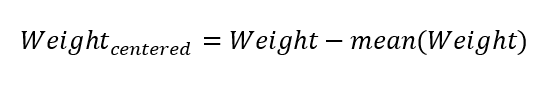
After centering, the mean of the new variable Weightcentered will be zero.
Centering a variable does not affect the model’s fit, so the R-squared and the residual standard deviation stay the same. However, the regression coefficient of that variable changes a lot.
Building the model with Weightcentered we get:
Cholesterol Level = β0 + β1 Weightcentered + ε
And the intercept can be interpreted as follows:
β0 is the estimated cholesterol level for a person with an average weight.
Standardizing the variable “Weight”:
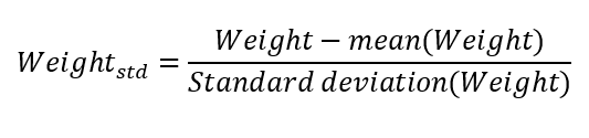
The second option would be to standardize Weight, i.e. to rescale it to have a mean of 0 and a standard deviation of 1. This is done by subtracting the mean and dividing by the standard deviation for each observation — thus obtaining Weightstd:
Building the model with Weightstd we get:
Cholesterol Level = β0 + β1 Weightstd + ε
Note that the coefficient β1 is now called the standardized coefficient of weight.
And the intercept can be interpreted in the same way as with centering:
β0 is the estimated cholesterol level for a person with an average weight.
Example 2: Interpreting main effects in a regression model with interaction
Now let’s add Age to our model with an interaction term Weight×Age:
Cholesterol Level = β0 + β1 Weight + β2 Age + β3 Weight×Age + ε
The challenge is to interpret the coefficients β1 and β2 i.e. the main effects of weight and age.
Let’s start with β1:
The simplest way to interpret β1 is to set Age = 0 in order to eliminate the terms Age and Age×Weight from the model, so the interpretation becomes:
β1 is the effect of weight on cholesterol, among the group where age = 0.
But since we do not expect our model to generalize to the subpopulation of newborns, it makes sense to either center or standardize the variable Age.
The same logic applies to the main effect of age (β2), since it cannot be interpreted with weight set to zero.
After centering (or standardizing) both Age and Weight, their coefficients will be:
β1: the effect of weight on cholesterol for an average aged person in our study.
And β2: the effect of age on cholesterol for a person with an average weight.
Technically, this interpretation will differ a little bit if we used centering instead of standardization.
For example, if weight is measured in Kilograms, after centering the variables, β1 can be interpreted as follows:
Among the subpopulation of average aged people, β1 will be the expected difference in cholesterol level comparing 2 groups who differ by 1 Kg in weight.
However, if we standardize them, β1 will be:
Among the subpopulation of average aged people, β1 will be the expected difference in cholesterol level comparing 2 groups who differ by 1 standard deviation in weight.
So centering produces a more intuitive interpretation, but as we will see in the next section, standardization still has the advantage of producing predictors whose effects can be compared with each other.
Standardizing predictors to assess their relative importance in the model
By standardizing the predictors in a regression model, the unit of measure of each becomes its standard deviation.
By measuring all variables in the model using the same unit, their regression coefficients become comparable, and therefore useful to assess their relative influence on the outcome.
For instance, the effect of a predictor will be twice as important as that of another one, if its standardized coefficient is twice as large.
This approach, however, has some limitations. If you are interested, I have a separate article on how to Assess Variable Importance in Linear and Logistic Regression.
Remember that this comparison should not be done when fitting the model using variables in their raw form (see: Standardized vs Unstandardized Regression Coefficients).
Non-linear transformations to improve model fit
Non-linear transformations such as log, square root, and polynomial transformations can help meet 3 important assumptions of linear regression:
- Linearity: A linear relationship must exist between the predictors and the outcome variable.
- Equal variance of the residuals: The error terms should have constant variance.
- Normality of the residuals: The residuals must follow a normal distribution.
The linearity and equal variance assumptions are important for inferential models — that is when using linear regression to study the relationship between X and Y. So violating them will lead to an incorrect estimation of the relationship between X and Y.
The linearity and normality assumptions are important for predictive purposes — that is when using linear regression to predict the outcome Y of new observations given their X values. So violating them will lead to a reduction in predictive accuracy.
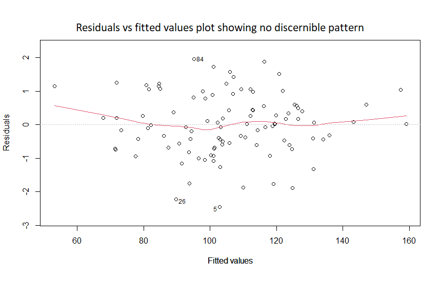
The linearity and the equal variance assumptions can both be checked by plotting the residuals versus fitted values.
For the linearity assumption:
The residuals versus fitted values should show no discernible pattern, as in the figure below:
If the plot shows a trend, such as a U-shape, then the linearity assumption is violated:
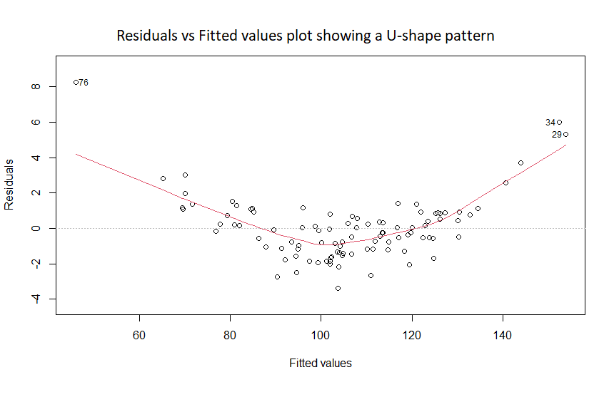
This can be corrected by using a non-linear transformation of the predictor variable X. For instance: log(X), √X, X2 or 1/X.
For the equal variance assumption:
If the plot of residuals versus fitted values shows a funnel-shape pattern, it is considered a sign of non-equal variance of the residuals:
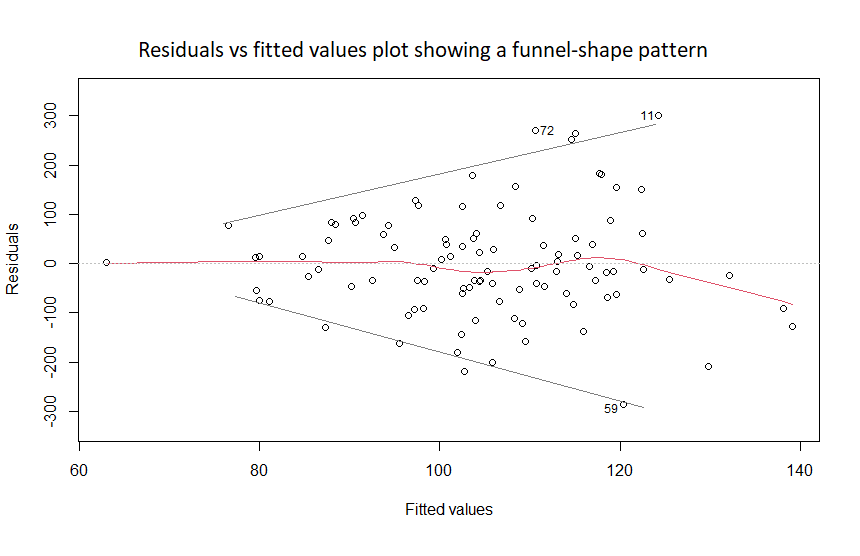
This can be corrected by using a non-linear transformation (logarithmic, polynomial, or square root) on the outcome variable Y.
The logarithmic and square root transformations make sense for variables with values that are all positive, such as: income, age, height, weight, etc.
The square root transformation produces uninterpretable regression coefficients, while the logarithmic transformation produces coefficients that can be interpreted in terms of percent changes instead of the raw units of the variable (see this article for more information).
For the normality of residuals assumption:
This assumption is violated if either:
1. The histogram of the residuals showed a non-bell shaped and asymmetric curve:

2. The Normal Q-Q plot of the residuals showed the data points not falling close to the straight line:
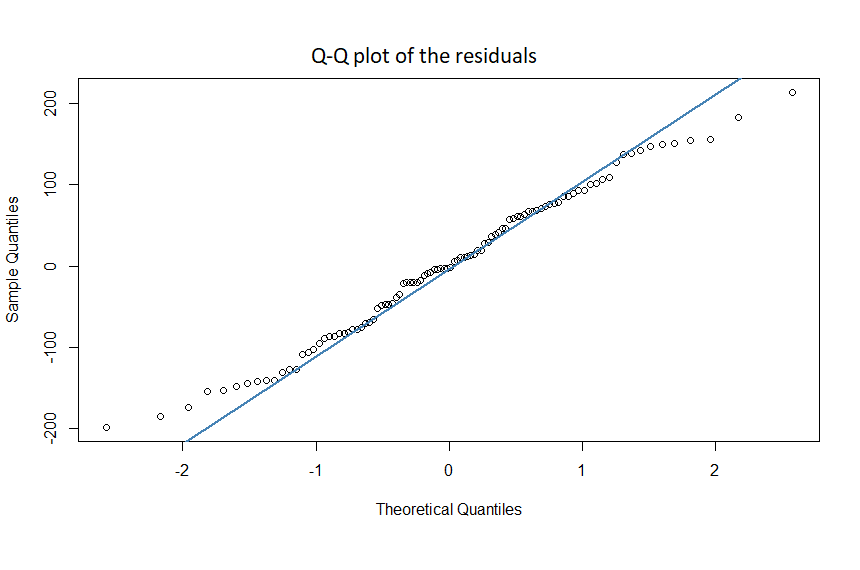
This violation can be corrected by applying a non-linear transformation on the predictor X or the outcome Y.
References
- Gelman A, Hill J, Vehtari A. Regression and Other Stories. Cambridge University Press; 2021.
- James G, Witten D, Hastie T, Tibshirani R. An Introduction to Statistical Learning with Applications in R.; 2021.