Here’s a table that summarizes the differences between correlation, collinearity and multicollinearity:
| Correlation | Collinearity | Multicollinearity | |
|---|---|---|---|
| Definition | Correlation refers to the linear relationship between 2 variables | Collinearity refers to a problem when running a regression model where 2 or more independent variables (a.k.a. predictors) have a strong linear relationship | Multicollinearity is a special case of collinearity where a strong linear relationship exists between 3 or more independent variables even if no pair of variables has a high correlation |
| Number of variables involved | 2 | 2 or more | 3 or more |
| Can be evaluated using | Correlation coefficient | Correlation matrix or VIF | VIF |
In this article, we’re going to discuss correlation, collinearity and multicollinearity in the context of linear regression:
Y = β0 + β1 × X1 + β2 × X2 + … + ε
One important assumption of linear regression is that a linear relationship should exist between each predictor Xi and the outcome Y. So, a strong correlation between these variables is considered a good thing.
However, when correlation exists between 2 predictors, we can no longer determine the effect of 1 while holding the other constant because the 2 variables change together. So their coefficients will become less exact and less interpretable.
The strong correlation between 2 independent variables will cause a problem when interpreting the linear model and this problem is referred to as collinearity.
In fact, collinearity is a more general term that also covers cases where 2 or more independent variables are linearly related to each other. So collinearity can exist either because a pair of predictors are correlated or because 3 or more predictors are linearly related to each other. This last case is sometimes referred to as multicollinearity.
Note that because multicollinearity is a special case of collinearity, some textbooks refer to both situations as collinearity such as: Regression Modeling Strategies by Frank Harrell and Clinical Prediction Models by Ewout Steyerberg. Others, such as An Introduction to Statistical Learning by Gareth James et al. prefer to make that distinction.
Correlation coefficient, correlation matrix, and VIF
The correlation coefficient r can help us quantify the linear relationship between 2 variables.
r is a number between -1 and 1 (-1 ≤ r ≤ 1):
- A value of r close to -1: means that there is negative correlation between the variables (when one increases the other decreases and vice versa)
- A value of r close to 0: indicates that the 2 variables are not correlated (no linear relationship exists between them)
- A value of r close to 1: indicates a positive linear relationship between the 2 variables (when one increases, so does the other)
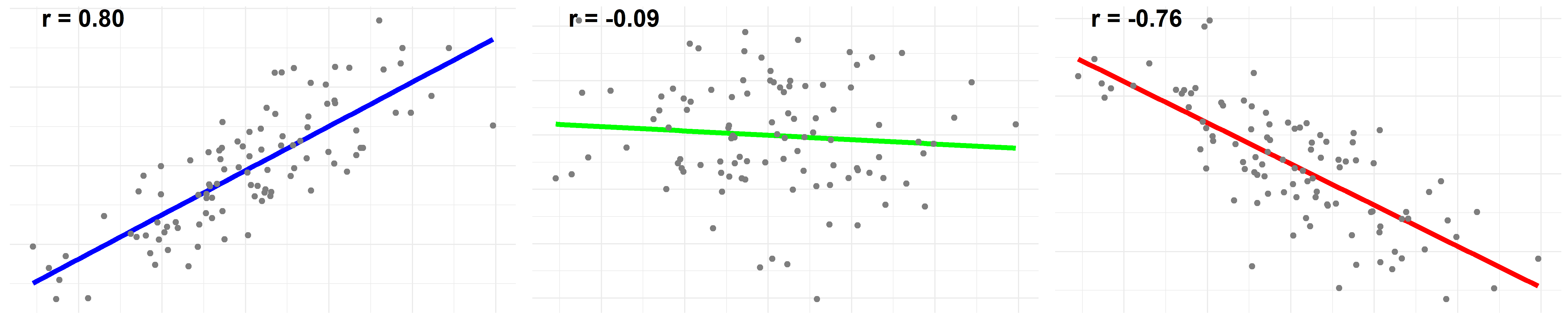
Here are 3 plots to visualize the relationship between 2 variables with different correlation coefficients. The first was drawn with a coefficient r of 0.80, the second -0.09 and the third -0.76:
When we have a linear model with multiple predictors (X1, X2, X3, …), we can compute the correlation coefficient for each pair and put it in a matrix.
This correlation matrix can help us identify collinearity. Here’s an example:
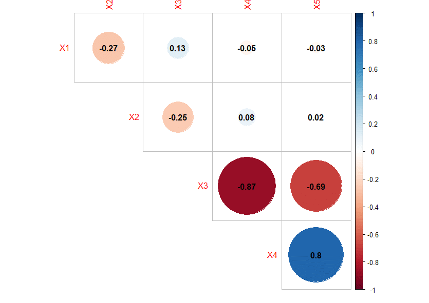
The correlation matrix above shows signs of collinearity as the absolute value of the correlation coefficients between X3-X4 and X4-X5 are above 0.7 [source].
However, because collinearity can also occur between 3 variables or more, EVEN when no pair of variables is highly correlated (a situation often referred to as “multicollinearity”), the correlation matrix cannot be used to detect all cases of collinearity.
This is where the variance inflation factor (VIF) comes to the rescue.
Here’s the formula for calculating VIF for the variable X1 in the model:
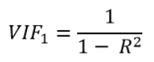
In this equation, R2 is the coefficient of determination from the linear regression model which has:
- X1 as dependent variable
- X2, X3, X4, … as independent variables
i.e. R2 comes from the following linear regression model:
X1 = β0 + β1 × X2 + β2 × X3 + β3 × X4 + … + ε
Because R2 is a number between 0 and 1:
- When R2 is close to 1 (X2, X3, X4, … are highly predictive of X1): the VIF will be very large
- When R2 is close to 0 (X2, X3, X4, … are not related to X1): the VIF will be close to 1
As a rule of thumb, a VIF > 10 is a sign of multicollinearity. However, this is somewhat an oversimplification. For more details on how to choose a threshold to detect multicollinearity and how to interpret a VIF value, I suggest my other article: What is an Acceptable Value for VIF?
Example: multicollinearity without correlation between any pair of predictors
In this section, we are going to work with simulated data. Here’s the R code if you want to follow along:
library(corrplot)
library(regclass)

# First define the predictors such that x5 is "slightly" related to all of the others
set.seed(1)
x1 = rnorm(100)
x2 = rnorm(100)
x3 = rnorm(100)
x4 = rnorm(100)
x5 = 0.1*x1 + 0.1*x2 + 0.1*x3 + 0.1*x4 + rnorm(100)*0.03

# y will be our depedent variable
y = rnorm(100)

# pack all the variables into a data frame
df = data.frame(X1=x1, X2=x2, X3=x3, X4=x4, X5=x5, Y=y)

# plot the correlation matrix
corrplot(cor(df[,c("X1", "X2", "X3", "X4", "X5")]), diag = FALSE, type="upper",addCoef.col = "black")

# then take a look at the VIF of each predictor
VIF(lm(Y ~ X1 + X2 + X3 + X4 + X5, data=df))
After running the code above, we get the following correlation matrix:
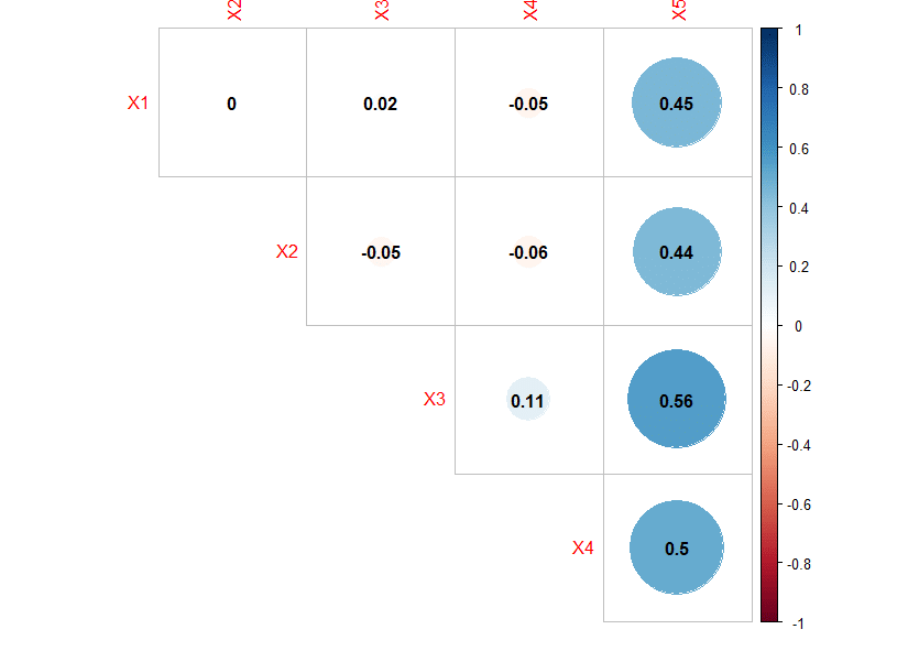
As you can see, the correlation matrix shows no sign of pairwise collinearity as all correlation coefficients are below 0.7.
However, looking at the VIF of each variable:

We see that 2 of them have a VIF > 10 signaling a multicollinearity problem.