Most research papers consider a VIF (Variance Inflation Factor) > 10 as an indicator of multicollinearity, but some choose a more conservative threshold of 5 or even 2.5.
So what threshold should YOU choose?
When choosing a VIF threshold, you should take into account that multicollinearity is a lesser problem when dealing with a large sample size compared to a smaller one. [Source]
That being said, here’s a list of references for different VIF thresholds recommended to detect collinearity in a multivariable (linear or logistic) model:
| VIF Threshold | Reference Type | Reference Date | Reference |
|---|---|---|---|
| VIF > 10 is problematic | Book | 2005 | Vittinghoff E. Regression Methods in Biostatistics: Linear, Logistic, Survival, and Repeated Measures Models. Springer; 2005. |
| VIF > 5 or VIF > 10 is problematic | Book | 2017 | James G, Witten D, Hastie T, Tibshirani R. An Introduction to Statistical Learning: With Applications in R. 1st ed. 2013, Corr. 7th printing 2017 edition. Springer; 2013. |
| VIF > 5 is cause for concern and VIF > 10 indicates a serious collinearity problem | Book | 2001 | Menard S. Applied Logistic Regression Analysis. 2nd edition. SAGE Publications, Inc; 2001. |
| VIF ≥ 2.5 indicates considerable collinearity | Research Paper | 2018 | Johnston R, Jones K, Manley D. Confounding and collinearity in regression analysis: a cautionary tale and an alternative procedure, illustrated by studies of British voting behaviour. Qual Quant. 2018;52(4):1957-1976. doi:10.1007/s11135-017-0584-6 |
How to interpret a given VIF value?
Consider the following linear regression model:
Y = β0 + β1 × X1 + β2 × X2 + β3 × X3 + ε
For each of the independent variables X1, X2 and X3 we can calculate the variance inflation factor (VIF) in order to determine if we have a multicollinearity problem.
Here’s the formula for calculating the VIF for X1:
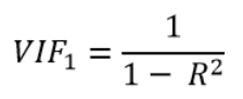
R2 in this formula is the coefficient of determination from the linear regression model which has:
- X1 as dependent variable
- X2 and X3 as independent variables
In other words, R2 comes from the following linear regression model:
X1 = β0 + β1 × X2 + β2 × X3 + ε
And because R2 is a number between 0 and 1:
- When R2 is close to 1 (i.e. X2 and X3 are highly predictive of X1): the VIF will be very large
- When R2 is close to 0 (i.e. X2 and X3 are not related to X1): the VIF will be close to 1
Therefore the range of VIF is between 1 and infinity.
Now, let’s discuss how to interpret the following cases where:
- VIF = 1
- VIF = 2.5
- VIF = +∞
Example 1: VIF = 1
A VIF of 1 for a given independent variable (say for X1 from the model above) indicates the total absence of collinearity between this variable and other predictors in the model (X2 and X3).
Example 2: VIF = 2.5
If for example the variable X3 in our model has a VIF of 2.5, this value can be interpreted in 2 ways:
- The variance of β3 (the regression coefficient of X3) is 2.5 times greater than it would have been if X3 had been entirely non-related to other variables in our model
- The variance of β3 is 150% greater than it would be if there were no collinearity effect at all between X3 and other variables in our model
Why 150%?
This percentage is calculated by subtracting 1 (the value of VIF if there were no collinearity) from the actual value of VIF:
2.5 – 1 = 1.5
In percent:
1.5 * 100 / 100 = 150%.
Example 3: VIF = Infinity
An infinite value of VIF for a given independent variable indicates that it can be perfectly predicted by other variables in the model.
Looking at the equation above, this happens when R2 approaches 1.