Plot Median and Interquartile Range in R

In this tutorial, we are going to create the following plot of the median and the interquartile range of sepal length for each iris species using the iris dataset:

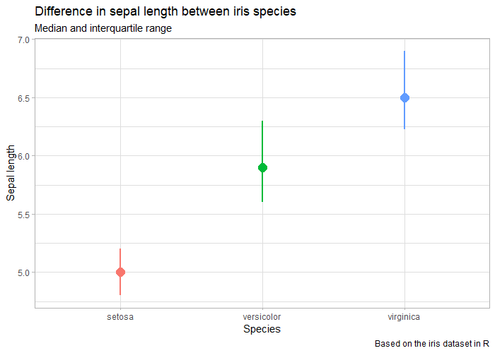
median and interquartile range of sepal length for different iris species

1. Using geom_pointrange()

We start by calculating the median, the 1st quartile, and the 3rd quartile as follows:

library(dplyr)

iris_summary <- iris |> 
  group_by(Species) |> 
  summarize(med = median(Sepal.Length),
            Q1 = quantile(Sepal.Length, 0.25),
            Q3 = quantile(Sepal.Length, 0.75))

iris_summary
## A tibble: 3 x 4
#  Species      med    Q1    Q3
#  <fct>      <dbl> <dbl> <dbl>
#1 setosa       5    4.8    5.2
#2 versicolor   5.9  5.6    6.3
#3 virginica    6.5  6.22   6.9

Then we give these variables to geom_pointrange() in ggplot2 and add some labels to the plot:

library(ggplot2)

ggplot(iris_summary, aes(x = Species, color = Species)) +
  geom_pointrange(aes(y = med,
                      ymin = Q1,
                      ymax = Q3),
                  show.legend = FALSE) +
  labs(y = 'Sepal length',
       title = 'Difference in sepal length between iris species',
       subtitle = 'Median and interquartile range',
       caption = 'Based on the iris dataset in R') +
  theme_light()

Output:

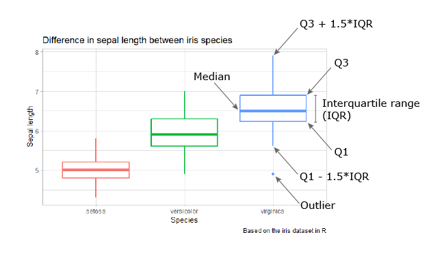
2. Using geom_boxplot()

Boxplots also show the median and the interquartile range, and can be plotted using the following code:

ggplot(iris, aes(x = Species, y = Sepal.Length, color = Species)) +
geom_boxplot(show.legend = FALSE) +
labs(y = 'Sepal length',
     title = 'Difference in sepal length between iris species',
     caption = 'Based on the iris dataset in R') +
theme_light()

Output:

boxplot showing the sepal length for different iris species

Here’s how to read a boxplot:

1. Using geom_pointrange()

2. Using geom_boxplot()

Further reading