In this tutorial, we will use the fpp3 library in R to manipulate and plot time series data. fpp3 loads other useful packages such as: dplyr, tidyr, lubridate, and ggplot2.
library(fpp3)
We will start with a simple example and then work with a more complicated one.
1. A simple time series example
1.1. Create the data
First, we will simulate some data (after setting the seed for reproducibility):
set.seed(1)

cancer <- data.frame(
  year = rep(2023, 12),
  month = 1:12,
  new_cases = sample(1:50, 12, replace = TRUE)
)

cancer
#   year month new_cases
#1  2023     1         4
#2  2023     2        39
#3  2023     3         1
#4  2023     4        34
#5  2023     5        23
#6  2023     6        43
#7  2023     7        14
#8  2023     8        18
#9  2023     9        33
#10 2023    10        21
#11 2023    11        21
#12 2023    12        42
Next, we will combine the variables year and month into 1 date variable:
# make_yearmonth() is available from fpp3
cancer <- cancer |>
  mutate(date = make_yearmonth(year, month)) |>
  select(-c(year, month)) # remove year and month

cancer
#   new_cases     date
#1          4 2023 Jan
#2         39 2023 Feb
#3          1 2023 Mar
#4         34 2023 Apr
#5         23 2023 May
#6         43 2023 Jun
#7         14 2023 Jul
#8         18 2023 Aug
#9         33 2023 Sep
#10        21 2023 Oct
#11        21 2023 Nov
#12        42 2023 Dec
1.2. Create a time series object
A time series table (i.e. a tsibble object) will make it easier for us to manipulate, analyze, and plot the time series data.
The function as_tsibble() requires us to specify the time index variable, which in this case is date:
cancer_ts <- as_tsibble(cancer,
                        index = date)

cancer_ts
## A tsibble: 12 x 2 [1M]
#   new_cases     date
#       <int>    <mth>
# 1         4 2023 Jan
# 2        39 2023 Feb
# 3         1 2023 Mar
# 4        34 2023 Apr
# 5        23 2023 May
# 6        43 2023 Jun
# 7        14 2023 Jul
# 8        18 2023 Aug
# 9        33 2023 Sep
#10        21 2023 Oct
#11        21 2023 Nov
#12        42 2023 Dec
The first line in the output (# A tsibble: 12 x 2 [1M]) is telling us that we have a time series table of 12 observations and 2 variables (12 × 2) which represent monthly data ([1M]).
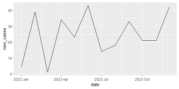
1.3. Plot time series
# 1st option
cancer_ts |>
  ggplot(aes(x = date, y = new_cases)) +
  geom_line()

# alternatively, we can use autoplot
autoplot(cancer_ts, new_cases)
Output:
2. A more complicated time series example
2.1. Create the data
In this second example, we will simulate time series data for 2 diseases: cancer and asthma.
set.seed(1)

diseases <- data.frame(
  year = rep(2023, 24), # 2 years
  month = rep(1:12, each = 2), # 2 years
  disease = rep(c("cancer", "asthma"), 12),
  new_cases = sample(1:50, 24, replace = TRUE)
)

diseases
#   year month disease new_cases
#1  2023     1  cancer         4
#2  2023     1  asthma        39
#3  2023     2  cancer         1
#4  2023     2  asthma        34
#5  2023     3  cancer        23
#6  2023     3  asthma        43
#7  2023     4  cancer        14
#8  2023     4  asthma        18
#9  2023     5  cancer        33
#10 2023     5  asthma        21
#11 2023     6  cancer        21
#12 2023     6  asthma        42
#13 2023     7  cancer        46
#14 2023     7  asthma        10
#15 2023     8  cancer         7
#16 2023     8  asthma         9
#17 2023     9  cancer        15
#18 2023     9  asthma        21
#19 2023    10  cancer        37
#20 2023    10  asthma        41
#21 2023    11  cancer        25
#22 2023    11  asthma        46
#23 2023    12  cancer        37
#24 2023    12  asthma        37
Next, we will combine the variables year and month into 1 date variable:
diseases <- diseases |>
  mutate(date = make_yearmonth(year, month)) |>
  select(-c(year, month)) # remove year and month

diseases
#   disease new_cases     date
#1   cancer         4 2023 Jan
#2   asthma        39 2023 Jan
#3   cancer         1 2023 Feb
#4   asthma        34 2023 Feb
#5   cancer        23 2023 Mar
#6   asthma        43 2023 Mar
#7   cancer        14 2023 Apr
#8   asthma        18 2023 Apr
#9   cancer        33 2023 May
#10  asthma        21 2023 May
#11  cancer        21 2023 Jun
#12  asthma        42 2023 Jun
#13  cancer        46 2023 Jul
#14  asthma        10 2023 Jul
#15  cancer         7 2023 Aug
#16  asthma         9 2023 Aug
#17  cancer        15 2023 Sep
#18  asthma        21 2023 Sep
#19  cancer        37 2023 Oct
#20  asthma        41 2023 Oct
#21  cancer        25 2023 Nov
#22  asthma        46 2023 Nov
#23  cancer        37 2023 Dec
#24  asthma        37 2023 Dec
2.2. Create time series object
Since we have observations for 2 diseases (cancer and asthma), i.e. for each date we have 2 rows, we will need to tell that to R by setting key = disease inside as_tsibble().
diseases_ts <- as_tsibble(diseases,
                          index = date,
                          key = disease)

diseases_ts
## A tsibble: 24 x 3 [1M]
## Key:       disease [2]
#   disease new_cases     date
#   <chr>       <int>    <mth>
# 1 asthma         39 2023 Jan
# 2 asthma         34 2023 Feb
# 3 asthma         43 2023 Mar
# 4 asthma         18 2023 Apr
# 5 asthma         21 2023 May
# 6 asthma         42 2023 Jun
# 7 asthma         10 2023 Jul
# 8 asthma          9 2023 Aug
# 9 asthma         21 2023 Sep
#10 asthma         41 2023 Oct
## ℹ 14 more rows
## ℹ Use `print(n = ...)` to see more rows
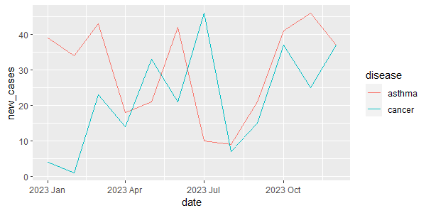
2.3. Plot time series
# 1st option
diseases_ts |>
  ggplot(aes(x = date, y = new_cases, color = disease)) +
  geom_line()

# alternatively, we can use autoplot()
autoplot(diseases_ts, new_cases)
Output: