For the following quadratic function:
\(f(x) = x^2 + 2x – 20\)
Here’s the plot that we want to produce:
Coding the function f(x) in R
A quadratic function is a function of the form: \(ax^2 + bx + c\), where \(a \neq 0\).
So for \(f(x) = x^2 + 2x – 20\):
- a = 1
- b = 2
- c = -20
In R, we write:
a = 1
b = 2
c = -20

f = function(x) {
  a*x^2 + b*x + c
}
Plotting the quadratic function f(x)
First, we have to choose a domain over which we want to plot f(x).
Let’s try -10 ≤ x ≤ 10:
# domain over which we want to plot f(x)
x = -10:10

# plot f(x)
plot(x, f(x), type = 'l') # type = 'l' plots a line instead of points

# plot the x and y axes
abline(h = 0)
abline(v = 0)
Output:

Finding the vertex
The vertex V of a quadratic equation, in this case the lowest point on the graph of f(x), is: \(V(\frac{-b}{2a}, f(\frac{-b}{2a}))\)
find.vertex = function(a, b, c) {
x_vertex = -b/(2 * a)
y_vertex = f(x_vertex)
c(x_vertex, y_vertex)
}
V = find.vertex(a, b, c)
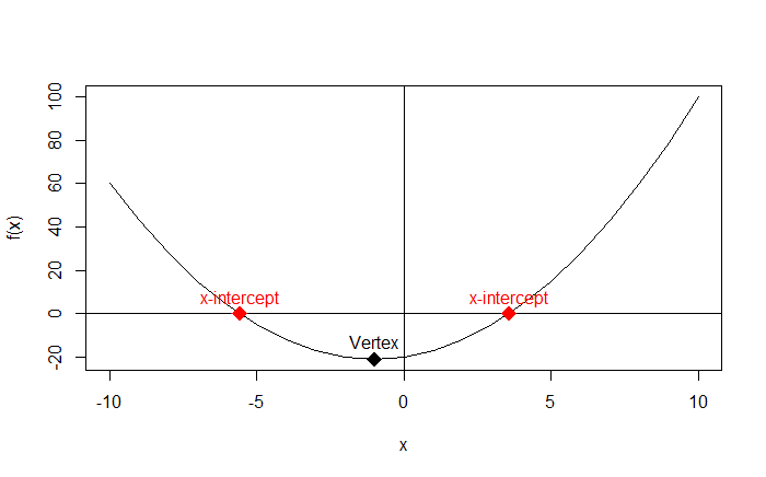
# print(V) outputs: -1 -21
# so the vertex is the point V(-1, -21)
Adding the vertex to the plot:
# add the vertex to the plot
points(x = V[1], y = V[2],
       pch = 18, cex = 2) # pch controls the form of the point and cex controls its size

# add a label next to the point
text(x = V[1], y = V[2],
     labels = "Vertex", pos = 3) # pos = 3 places the text above the point
Output:

Finding the x-intercepts of f(x)
The x-intercepts are the solutions of the quadratic equation f(x) = 0; they can be found by using the quadratic formula:
\(x = \frac{-b \pm \sqrt{b^2 – 4ac}}{2a}\)
The quantity \(b^2 – 4ac\) is called the discriminant:
- if the discriminant is positive, then f(x) has 2 solutions (i.e. 2 x-intercepts).
- if the discriminant is zero, then f(x) has 1 solution (i.e. 1 x-intercept).
- if the discriminant is negative, then f(x) has no real solutions (i.e. does not intersect the x-axis).
# find the x-intercepts of f(x)
find.roots = function(a, b, c) {
  discriminant = b^2 - 4 * a * c
  if (discriminant > 0) {
    c((-b - sqrt(discriminant))/(2 * a), (-b + sqrt(discriminant))/(2 * a))
  }
  else if (discriminant == 0) {
    -b / (2 * a)
  }
  else {
    NaN
  }
}

solutions = find.roots(a, b, c)

# print(solutions) outputs: -5.582576  3.582576
# so the x-intercepts are the points: (-5.582576, 0) and (3.582576, 0)
Adding the x-intercepts to the plot:
# add the x-intercepts to the plot
points(x = solutions, y = rep(0, length(solutions)), # x and y coordinates of the x-intercepts
       pch = 18, cex = 2, col = 'red')

text(x = solutions, y = rep(0, length(solutions)),
     labels = rep("x-intercept", length(solutions)),
     pos = 3, col = 'red')
Output:
Here’s the full code used in this tutorial
a = 1
b = 2
c = -20

f = function(x) {
  a*x^2 + b*x + c
}

# simple plot of f(x)
x = -10:10
plot(x, f(x), type = 'l')

# plot the x and y axes
abline(h = 0)
abline(v = 0)


# find the vertex
find.vertex = function(a, b, c) {
  x_vertex = -b/(2 * a)
  y_vertex = f(x_vertex)
  c(x_vertex, y_vertex)
}

V = find.vertex(a, b, c)

# add the vertex to the plot
points(x = V[1], y = V[2],
       pch = 18, cex = 2)

text(x = V[1], y = V[2],
     labels = "Vertex", pos = 3)


# find the x-intercepts of f(x)
find.roots = function(a, b, c) {
  discriminant = b^2 - 4 * a * c
  if (discriminant > 0) {
    c((-b - sqrt(discriminant))/(2 * a), (-b + sqrt(discriminant))/(2 * a))
  }
  else if (discriminant == 0) {
    -b / (2 * a)
  }
  else {
    NaN
  }
}

solutions = find.roots(a, b, c)

# add the x-intercepts to the plot
points(x = solutions, y = rep(0, length(solutions)),
       pch = 18, cex = 2, col = 'red')

text(x = solutions, y = rep(0, length(solutions)),
     labels = rep("x-intercept", length(solutions)),
     pos = 3, col = 'red')
I encourage you to play with this code, for example, you can change the function f(x) to get a negative discriminant, by using:
- a = 1
- b = 2
- c = 2
What does the plot look like in this case?