In this article, will use the uniroot.all() function from the rootSolve package to find all the solutions of an equation over a given interval (or domain).
Input: uniroot.all() takes 2 arguments: a function f and an interval.
How it works: Its searches the interval for all possible roots of f.
Output: uniroot.all() returns a vector of all roots of f over the interval.
Here are some examples:
1. Find the solution of a simple function: \(|x| + 4 = 0\)
First we enter the function in R:
library(rootSolve)

# writing the function
f1 = function(x) {
  abs(x) - 4
}
Next, we plot the function to try to determine visually how many solutions it has (i.e. where and how many times it crosses the line y = 0). This will help us define an interval (domain) over which we will search for a solution.
# let's try plotting the function
# over the range [-50, 50]
x = -50:50
plot(x, f1(x), type = 'l')

# adding a horizontal line at y = 0
abline(h = 0, col = 'blue')
Output:
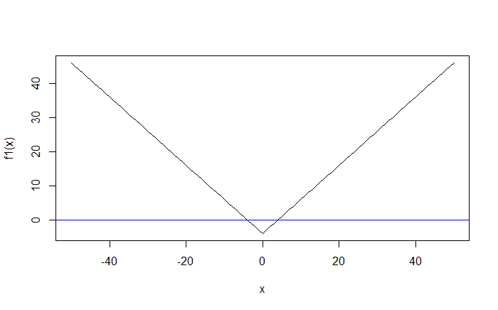
So we see that the function crosses the blue line at 2 points, and that the domain [-50, 50] covers all the solutions of the function f.
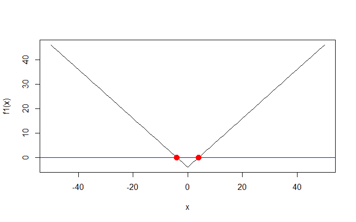
Next, we will use uniroot.all() to find all the solutions of f over [-50, 50]
roots = uniroot.all(f1, c(-50, 50))

# print(roots) outputs: -4  4

# graphing the roots of f1
points(x = roots, y = rep(0, length(roots)), col = "red", pch = 16, cex = 1.5)
Output:
2. Find the solution of a more complex function: \(\frac{\sqrt{x}}{(x + 2)} – \frac{1}{4} = 0\)
library(rootSolve)

# writing the function
f2 = function(x) {
  sqrt(x) / (x + 2) - 1/4
}
Next, we will plot the function over the interval [0, 100] (since it contains \(\sqrt{x}\), it doesn’t make sense to try negative values).
# let's try plotting the function
# over the range [0, 100]
x = 0:100
plot(x, f2(x), type = 'l')

# adding a horizontal line at y = 0
abline(h = 0, col = 'blue')
Output:
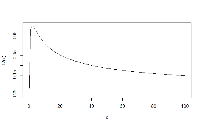
We see that the function f has 2 solutions in the domain [0,100].
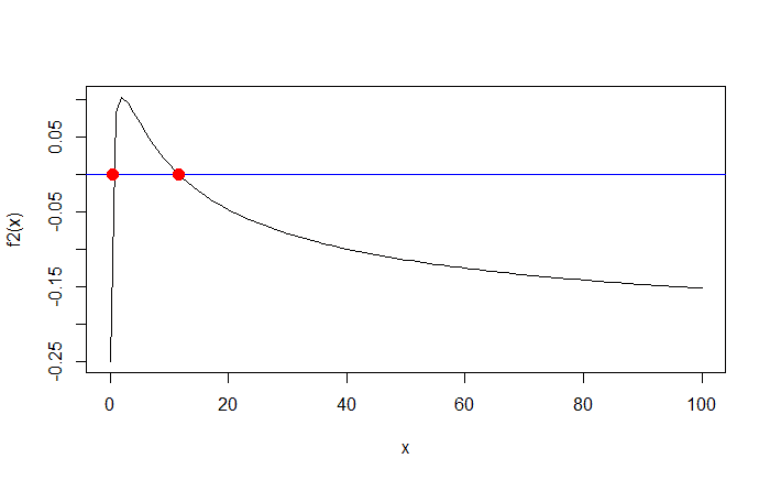
Let’s find exactly what they are:
uniroot.all(f2, c(0, 100))

# outputs: 0.3431545 11.6568502

# let's plot the solutions
points(x = roots, y = rep(0, length(roots)), col = "red", pch = 16, cex = 1.5)
Output:
3. Find the solution of the function: \(\frac{1}{x} = 0\)
This example shows that uniroot.all() has some imperfections. Sometimes it cannot find all the roots over the specified interval, and sometimes it even outputs a wrong answer.
library(rootSolve)

# writing the function
f3 = function(x) {
  1 / x
}
Plotting the function over the domain [-50, 50].
x = -50:50
plot(x, f3(x), type = 'l')
abline(h = 0, col = 'blue')
Output:
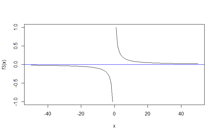
We see that \(\frac{1}{x} = 0\) does not have any solutions.
Anyway, let’s run uniroot.all() on f3:
# finding the roots of f3
roots = uniroot.all(f3, c(-50, 50))

# print(roots) outputs: -0.0004884619

# plotting the roots of f3
points(x = roots, y = rep(0, length(roots)), col = "red", pch = 16, cex = 1.5)
Output:
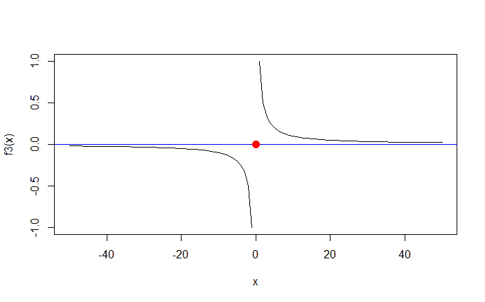
In conclusion, you should always plot the function and its solutions to make sure that the solution(s) outputted by uniroot.all() make sense.