Weighted regression (a.k.a. weighted least squares) is a regression model where each observation is given a certain weight that tells the software how important it should be in the model fit.
Weighted regression can be used to:
- Handle non-constant variance of the error terms in linear regression.
- Handle variability in measurement accuracy.
- Account for sample misrepresentation.
- Account for duplicate observations.
1. Weighted regression to handle non-constant variance of error terms
Linear regression assumes that the error terms have constant variance (i.e. are homoscedastic).
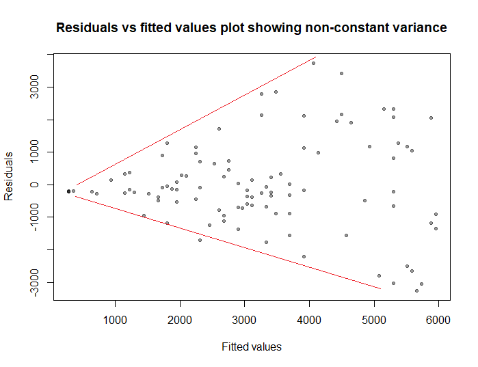
We can check this assumption by plotting the residuals of the model versus the fitted values. If the plot shows a funnel shape (see figure below), we conclude that the variance is not constant and the assumption of homoscedasticity is violated.
In this case, we can use weighted regression where we impose less weight on the part of the data where the variance is high, and more weight on the part where the variance is low.
Example:
Suppose we want to study the relationship between the number of hours worked per week and the monthly salary. So we plot the relationship between the two:
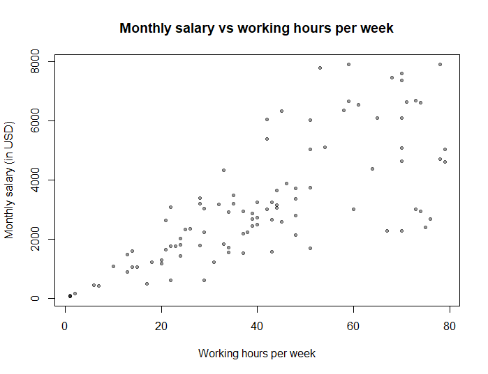
As expected, the more people work, the higher their income. But notice that as the number of worked hours increases, the variance in the salary also increases: this is because the salary of those who work 0 hours will definitely be 0$ (no variance), but the salary of those who work 80 hours per week will likely be somewhere between 2000 and 8000$ per month (high variance).
If we use linear regression to predict the Monthly salary using Working hours, the residuals will show the following funnel shape:

So the homoscedasticity assumption of ordinary linear regression is violated (which will bias the standard errors of the regression coefficients, the confidence intervals, and the p-values).
In order to handle non-constant variance of the residuals, we can use a weighted regression model, with weights that are inversely proportional to the variance of monthly salary.
\(Weights = \frac{1}{\text{variance of monthly salary}}\)
Now we will have to guess the variance of monthly salary for different values of working hours. Our best guess of this variance is to regress the absolute values of the residuals against the fitted values, and the resulting fitted values squared of this regression will be our estimates of this variance.
In R we run the following code:
# ordinary linear regression model
model = lm(monthlySalary ~ workingHours)

# estimating the variance of monthly salary
variance = lm(abs(model$residuals) ~ model$fitted.values)$fitted.values^2

# calculating the weights
weights = 1 / variance

# weighted regression model
weighted_model = lm(monthlySalary ~ workingHours, weights = weights)
The plot below shows in red the observations associated with higher weights and in blue those associated with lower weights:
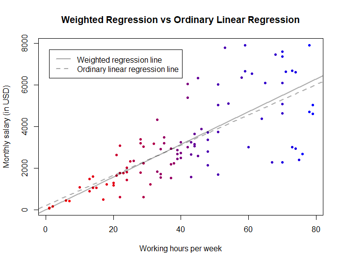
Notice how the red points to the left (with very high weights) force the weighted regression line to pass through them, unlike the ordinary linear regression line that passes above them. Here, weighted regression is better because it models the fact that we are more certain about the Y-values of these red points (i.e. the fact that if you work 0 hours per week, you certainly get 0$ per month; but if you work 80 hours per week, we will be less certain about your salary).
2. Weighted regression to handle variability in measurement accuracy
Weighted regression can be used to weight observations by confidence — by giving lower weights to less reliable data points and higher weights for observations that are more precise.
Example 1:
Sometimes observations are measured with different instruments that do not have the same accuracy. In these cases, we can use weights to give more importance to the more accurate measurements.
Here the weights must be chosen according to our knowledge about the accuracy of the instruments.
Example 2:
In some studies, older observations are less precise than newer ones. In these cases for instance, we want observations collected in 2022 to have more weight than those collected in 2010.
So for example, if data collection started in 2001, then each observation can be weighted by the number of years since 2000:
\(Weights = Year – 2000\)
(So an observation in 2001 will have a weight of 1, another observation in 2005 will have a weight of 5, etc.)
In practice, before running the weighted regression model, we scale the variable weights to have an average of 1, by dividing it by its average:
\(Weights = \frac{Weights}{mean(Weights)}\)
3. Weighted regression to account for sample misrepresentation
Some surveys have very complex sampling designs that involve unequal selection probability. In these cases, certain subgroups of the population tend to be misrepresented (for example, the study may end up with a higher proportion of males than the population, or a different distribution of age than the population).
This problem can be solved by applying higher weights for the observations that are less represented in the sample, and lower weights for the observations that are overrepresented. Using weighted regression in this context will produce more generalizable estimates.
Example:
The NHANES, a survey conducted to assess the health and nutritional status of people in the US, does not use simple random sampling. Instead, it has a complex sampling design that requires the use of weights to account for the unequal probability of unit selection.
In this context, weighted regression produces estimates that better resemble the population by accounting for sample misrepresentation. (for more information on how to calculate the weights for NHANES data, see this page from cdc.gov)
4. Weighted regression to account for duplicate observations
In cases where each row in the data represents multiple observations (that have the same values), then weighted regression on this dataset will be equivalent to an ordinary regression on the original dataset (where each row represents only 1 observation).
Example
The HairEyeColor dataset in R is an example of a compressed dataset where each row represents more than 1 observation:
# load the dataset as an R data frame
dat = as.data.frame(HairEyeColor)
Here are the first 5 rows of this dataset:
| Row # | Hair Color | Eye Color | Gender | Frequency |
|---|---|---|---|---|
| 1 | Black | Brown | Male | 32 |
| 2 | Brown | Brown | Male | 53 |
| 3 | Red | Brown | Male | 10 |
| 4 | Blond | Brown | Male | 3 |
| 5 | Black | Blue | Male | 11 |
The first row represents 32 observations, the second row represents 53 observations, and so on…
Suppose we want to run a logistic regression model to predict the value of Gender using Eye Color.
We have 2 options:
Option 1: We can run a weighted regression model on the compressed dataset that we have, weighting by the variable Frequency:
# run weighted logistic regression on the compressed dataset that we have
summary(glm(Sex ~ Eye, family = 'binomial', data = dat, weights = Freq))

# Call:
# glm(formula = Sex ~ Eye, family = "binomial", data = dat, weights = Freq)
#
# Deviance Residuals:
#     Min       1Q   Median       3Q      Max
# -9.2584  -3.9208  -0.1454   3.3859   9.0116
#
# Coefficients:
#             Estimate Std. Error z value Pr(>|z|)
# (Intercept)  0.21905    0.13565   1.615    0.106
# EyeBlue     -0.09798    0.19254  -0.509    0.611
# EyeHazel    -0.24056    0.24782  -0.971    0.332
# EyeGreen    -0.28157    0.28454  -0.990    0.322
#
# (Dispersion parameter for binomial family taken to be 1)
#
#     Null deviance: 818.73  on 31  degrees of freedom
# Residual deviance: 817.20  on 28  degrees of freedom
# AIC: 825.2
#
# Number of Fisher Scoring iterations: 3
Option 2: We can also get the same regression output by recovering the original dataset (by repeating each row according to the value of Frequency) and then run the logistic regression model:
# recover the original dataset
original.dat = dat[,-4][rep(1:nrow(dat), dat$Freq),]

# run unweighted logistic regression on the original dataset
summary(glm(Sex ~ Eye, family = 'binomial', data = original.dat))

# Call:
# glm(formula = Sex ~ Eye, family = "binomial", data = original.dat)
#
# Deviance Residuals:
#    Min      1Q  Median      3Q     Max
# -1.272  -1.229   1.086   1.126   1.204
#
# Coefficients:
#             Estimate Std. Error z value Pr(>|z|)
# (Intercept)  0.21905    0.13565   1.615    0.106
# EyeBlue     -0.09798    0.19254  -0.509    0.611
# EyeHazel    -0.24056    0.24782  -0.971    0.332
# EyeGreen    -0.28157    0.28454  -0.990    0.322
#
# (Dispersion parameter for binomial family taken to be 1)
#
#     Null deviance: 818.73  on 591  degrees of freedom
# Residual deviance: 817.20  on 588  degrees of freedom
# AIC: 825.2
#
# Number of Fisher Scoring iterations: 3
References
- Huntington-Klein N. The Effect. 1st edition. Routledge; 2022.
- Gelman A, Hill J, Vehtari A. Regression and Other Stories. 1st edition. Cambridge University Press; 2020.
- James G, Witten D, Hastie T, Tibshirani R. An Introduction to Statistical Learning: With Applications in R. 2nd ed. 2021 edition. Springer; 2021.
- Bruce P, Bruce A, Gedeck P. Practical Statistics for Data Scientists: 50+ Essential Concepts Using R and Python. 2nd edition. O’Reilly Media; 2020.