Linear regression has 4 assumptions:
- Linearity: The relationship between each predictor Xi and the outcome Y should be linear.
- Independence of errors: Each observation is drawn randomly from the population.
- Constant variance of errors: The dispersion of the data points around the regression line should be constant.
- Normality of errors: Error terms should be normally distributed.
1. How to check linearity
Instead of checking the relationship between each predictor and the outcome in a multivariable model, we can plot the residuals versus the fitted values. The plot should show no discernible pattern:
model = lm(y ~ x)

# plot the residuals vs fitted values
plot(model, 1)
The output will look like one of the following:
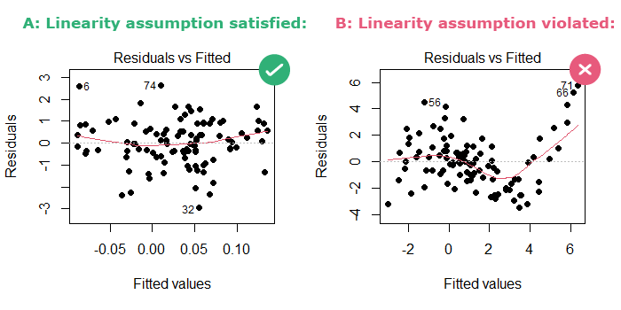
In this plot, R draws a LOESS red line that smoothly fits the data:
- In part A: The LOESS line looks like “a child’s freehand drawing of a straight line” [Cohen et al., 2002], so the linearity assumption is satisfied.
- In part B: the LOESS line is curved, so the linearity assumption is violated.
2. How to check the independence of errors
The second assumption of linear regression is that errors are not correlated with each other.
Remember that, in linear regression:
- An error is the distance between an observed data point and the true population value, which is unmeasurable.
- A residual, however, is the distance between an observed data point and the linear regression line. It estimates the error and it is measurable.
Therefore, we can use residuals instead of errors to check the assumptions of a linear regression model. In this case, the independence of errors assumption means that the residuals should not be correlated.
Here are some examples of settings where residuals might be correlated:
- In time series data: where correlation happens because the same participants are measured repeatedly over time (people tend to be correlated with themselves).
- In cluster samples: where correlation happens because some participants in the study are relatives and/or live in a similar geographical place (these people tend to be correlated with each other).
In both of these cases, methods other than simple linear regression should be used to analyze the data.
Instead, if the data are a simple random sample of the population, then the errors will be independent (i.e. the assumption will be satisfied).
Therefore, checking this assumption involves understanding the study design and the data collection process which will help choose the appropriate statistical method to analyze the data.
3. How to check the constant variance of errors
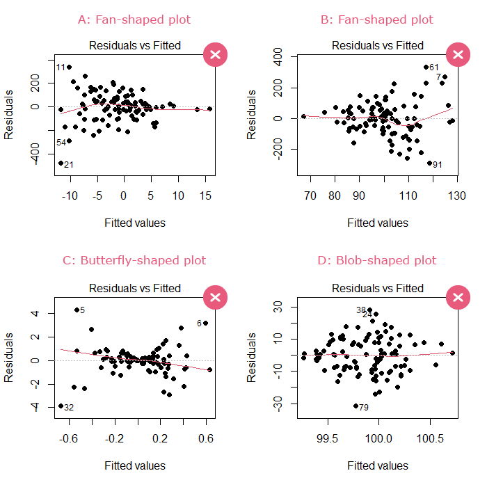
Plot the residuals versus fitted values:
- If the points are scattered and show no discernible shape: then this assumption is satisfied.
- If the points show a fan, butterfly, or blob shape: then this assumption is violated.
model = lm(y ~ x)

# plot the residuals vs fitted values
plot(model, 1)
The output should not look like one of the following:
When X is a categorical predictor, the plot of the residuals vs fitted values will not be helpful as much. Here’s an example:

So for categorical predictors we need another way to check the assumption of constant variance of errors.
Huntington-Klein recommends the following:
Calculate the variance of the residuals for each subgroup of the predictor X. The constant variance assumption will be violated if the variance of the residuals:
- Changes by a factor of 2 or more between subgroups that differ in size by a factor of 2 or more.
- Changes by a factor of 3 or more between subgroups that differ in size by a factor of less than 2.
Here’s the R code to do it:
# calculate the residuals variance for each subgroup of x
tapply(model$residuals, x, var)
#         0         1
# 1.0697939 0.7184118

# sample size in each subgroup of x
table(x)
#  0  1
# 49 51
Conclusion: the 2 subgroups of X (0 and 1) are similar in size (49 vs 51 observations in each) and differ only by a factor of ~1.5 (1.0697939/0.7184118 = 1.48911) in the variance of the residuals, which is less than 3, so we can assume that the errors have constant variance.
Statistical tests are sensitive to sample sizes: in small samples they do not have enough power to reject the null, and therefore will give a false sense of reassurance. Also, instead of getting a pass/fail answer from a statistical test, we need to examine the severity of the violation of the constant variance assumption [source: Vittinghoff et al., 2011]
4. How to check the normality of errors
The normality of error terms is a problem in 2 cases only: (1) in small sample sizes [Vittinghoff et al., 2011] and (2) when using linear regression for prediction purposes as opposed to estimating the relationship between a predictor X and an outcome Y [Gelman et al., 2020].
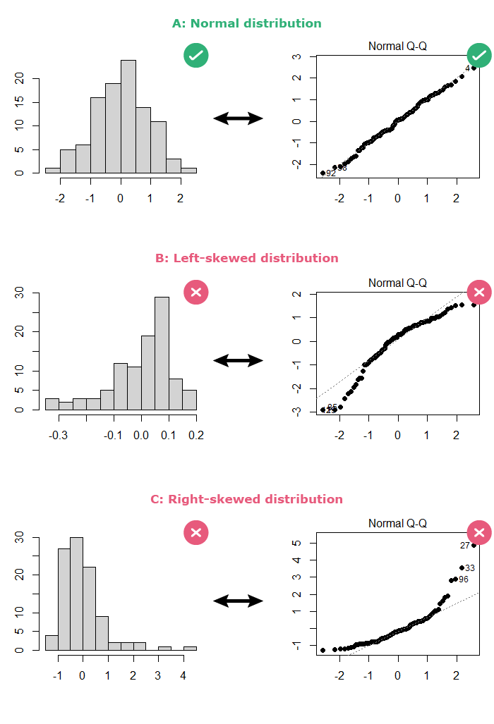
The normality of errors can be checked in 2 ways:
- By looking at a histogram of the residuals: the distribution should be bell-shaped.
- By looking at a normal Q-Q plot of the residuals: The points should follow the diagonal straight line.
# plot side by side
par(mfrow=c(1,2))

hist(model$residuals)
plot(model, 2)
If the residuals are normally distributed, your output should look like part A below:
Statistical tests are sensitive to sample sizes:
- In small samples, where the assumption of normality is most important for linear regression, they do not have enough power to reject the null.
- In large samples, where linear regression is robust regarding departure from normality, they reject the null for a small departure from normality.
Linear regression does not require the outcome Y (nor the predictor X) to be normally distributed. Only errors should be normally distributed, and they can be even when Y is not.
References
- Cohen J, Cohen P, West SG, Aiken LS. Applied Multiple Regression/Correlation Analysis for the Behavioral Sciences, 3rd Edition. Third edition. Routledge; 2002.
- Vittinghoff E, Glidden DV, Shiboski SC, McCulloch CE. Regression Methods in Biostatistics: Linear, Logistic, Survival, and Repeated Measures Models. 2nd ed. 2012 edition. Springer; 2011.
- Huntington-Klein N. The Effect. 1st edition. Routledge; 2022.
- Gelman A, Hill J, Vehtari A. Regression and Other Stories. 1st edition. Cambridge University Press; 2020.