The most important assumption of linear regression is that the relationship between each predictor and the outcome is linear.
When the linearity assumption is violated, try:
- Adding a quadratic term to the model
- Adding an interaction term
- Log transforming a predictor
- Categorizing a numeric predictor
Let’s create some non-linear data to demonstrate these methods:
set.seed(2)
# creating the variables:
# age
age = rnorm(n = 100, mean = 50, sd = 10)

# ldl cholesterol
ldl = rnorm(n = 100, mean = 120, sd = 35)

# systolic blood pressure
sbp = 0.01*age^2 - 3*log(age) + 2*sqrt(ldl) + rnorm(100, 90, 10)

model1 = lm(sbp ~ age + ldl)

# plotting residuals vs fitted values
plot(model1, 1)
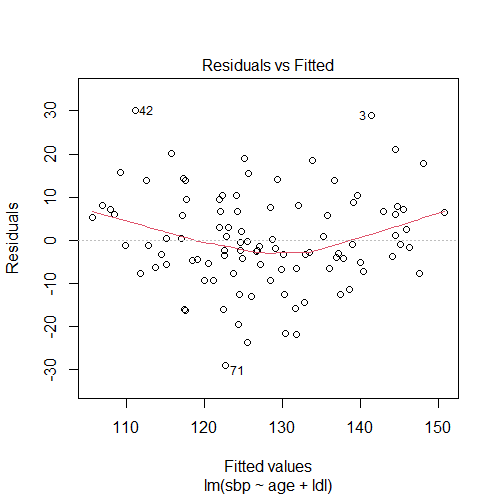
The residuals vs fitted values plot shows a curved relationship, therefore, the linearity assumption is violated.
Solution #1: Adding a quadratic term
Non-linearity may be fixed by adding age2 and/or ldl2 to our model. We can check if this solution works by:
- Using ANOVA to compare the model with a quadratic term with the model without a quadratic term (the null hypothesis is that the two models fit the data equally well, and the alternative hypothesis is that the model with a quadratic term is superior).
- Comparing the adjusted-R2 of the model with a quadratic term with that of the model without a quadratic term.
- Plotting the residuals versus the fitted values for the model with a quadratic term.
Adding age2
# adding age-squared
model2 = lm(sbp ~ age + I(age^2) + ldl)
# note the use of the I() function, since age^2 alone has another meaning in R

# checking our solution
#1. comparing models with ANOVA and getting the p-value
anova(model1, model2)['Pr(>F)'][2,] # 4.983351e-05

#2. comparing the adjusted R-squared
summary(model1)$adj.r.squared # 0.4807024
summary(model2)$adj.r.squared # 0.5583325

#3. plotting residuals vs fitted values for the new model
plot(model2, 1)
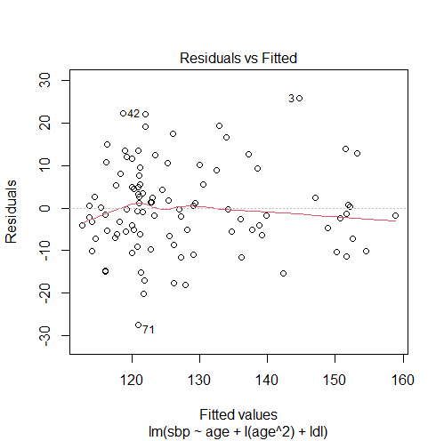
From these results, we can conclude that adding age2 fixed the violation of the linearity assumption since:
- The p-value of the ANOVA is 4.983e-05 (< 0.05), which means that the model containing age2 fits the data better.
- The adjusted-R2 of the model with age2 is higher.
- The non-linear pattern in the residuals vs fitted values plot disappeared.
Adding ldl2
# adding ldl-squared
model3 = lm(sbp ~ age + I(age^2) + ldl + I(ldl^2))

# checking our solution
#1. comparing models with ANOVA and getting the p-value
anova(model2, model3)['Pr(>F)'][2,] # 0.9640057

#2. comparing the adjusted R-squared
summary(model2)$adj.r.squared # 0.5583325
summary(model3)$adj.r.squared # 0.5536929
Adding another quadratic term (ldl2) does not improve model2 since:
- The p-value of the ANOVA is > 0.05, which means that the model containing ldl2 does not fit the data better than model2.
- The adjusted-R2 of the model with ldl2 is approximately the same as model2.
(For more information, see: Why Add & How to Interpret a Quadratic Term in Regression)
Solution #2: Adding an interaction term
Since non-linearity may be due to an interaction between predictors, we can try adding an interaction term between the predictors: age and ldl:
model4 = lm(sbp ~ age + ldl + age:ldl)

# checking our solution
#1. comparing models with ANOVA and getting the p-value
anova(model3, model1)['Pr(>F)'][2,] # 0.3097294

#2. comparing the adjusted R-squared
summary(model1)$adj.r.squared # 0.4807024
summary(model4)$adj.r.squared # 0.4809317

#3. plotting residuals vs fitted values for the new model
plot(model4, 1)
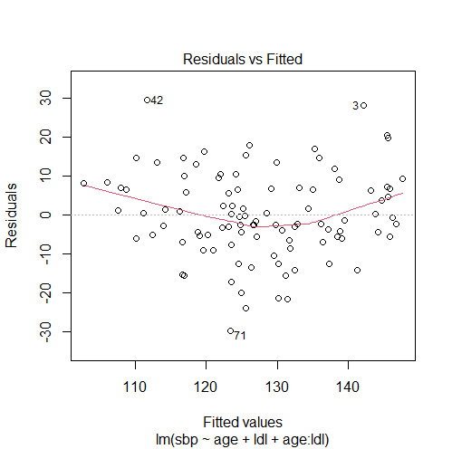
These results suggest that adding an interaction term does not fix the violation of the linearity assumption since the model with interaction:
- Did not fit the data better (ANOVA p-value > 0.05).
- Does not have a higher adjusted-R2.
- Also has a non-linearity pattern in the residuals vs fitted values plot.
(For more information, see: Why and When to Include Interactions? and Interpret Interactions in Linear Regression)
Solution #3: Transforming a predictor variable
Next, we can try using a log or a square root transformation of the predictors age and/or ldl.
The difference is that with a log transformation the model will still be interpretable, so this is what we are going to use here (for more information, see: Interpret Log Transformations in Linear Regression):
Log transforming age:
model5 = lm(sbp ~ log(age) + ldl)

# checking our solution
#1. comparing the adjusted R-squared
summary(model1)$adj.r.squared # 0.4807024
summary(model5)$adj.r.squared # 0.4164599

#2. plotting residuals vs fitted values for the new model
plot(model5, 1)
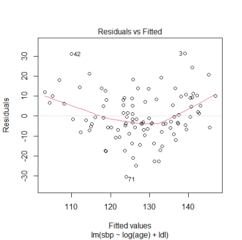
The results show that replacing age with log(age) does not fix the violation of the linearity assumption since:
- It did not improve the model’s adjusted-R2.
- It did not eliminate the non-linearity pattern in the residuals vs fitted values plot.
Log transforming ldl:
model6 = lm(sbp ~ age + log(ldl))

# checking our solution
#1. comparing the adjusted R-squared
summary(model1)$adj.r.squared # 0.4807024
summary(model6)$adj.r.squared # 0.4819157

#2. plotting residuals vs fitted values for the new model
plot(model6, 1)

Also replacing ldl with log(ldl) does not fix the violation of the linearity assumption since:
- It only provided a tiny improvement in the model’s adjusted-R2.
- It did not eliminate the non-linearity pattern in the residuals vs fitted values plot.
Solution #4: Categorizing a numeric predictor
When other solutions fail, we can handle non-linearity by categorizing a numeric predictor according to cutpoints that make sense theoretically.
Here, for the sake of demonstration, we will not waste time with choosing the perfect cutpoints, so we will categorize both age and ldl by dividing them into 3 categories:
Categorizing age
# divide age into 3 categories
age_cat = cut(age, breaks = 3)

model7 = lm(sbp ~ age_cat + ldl)

# checking our solution
summary(model1)$adj.r.squared # 0.4807024
summary(model7)$adj.r.squared # 0.4936364
Since the adjusted-R2 improved, we will keep the categorical version of age, and try categorizing ldl as well:
Categorizing ldl
# divide ldl into 3 categories
ldl_cat = cut(ldl, breaks = 3)

model8 = lm(sbp ~ age_cat + ldl_cat)

# checking our solution
summary(model7)$adj.r.squared # 0.4936364
summary(model8)$adj.r.squared # 0.5146501
Categorizing ldl also provided us with a better model since it improved the adjusted-R2.