Suppose we are interested in studying whether smoking increases heart rate.

Because it would not be ethical to randomly assign people to smoke, we are stuck with an observational design where we have to deal with bias and confounding ourselves.
The questions that we are going to be concerned with in this article are:
Which factors have the potential to confound the relationship between smoking and heart rate? and how to control for these factors?
Coming up with a list of potential confounders
A confounding variable is a common cause of both the exposure (smoking) and the outcome (heart rate).
(If you want to know why I chose this definition of a confounding variable, I have a separate article where I discuss and evaluate 4 different methods to identify confounding.)
To make things easier at this early stage of the analysis, let’s forget about causality for now and list all factor that we think might be associated with both the exposure and the outcome.
For example:
- Coffee consumption: It is well known that coffee consumers tend to be smokers, so any information about whether someone drinks coffee or not must be associated with smoking. Also, coffee contains caffeine which increases heart rate. So coffee is a good confounding candidate.
- Adrenaline level: Adrenaline is a known marker of stress, and some people may smoke to ease that stress, so adrenaline might be associated with smoking. Also adrenaline is certainly associated with an elevated heart rate. So adrenaline level is another confounding candidate.
Many other factors may also confound the relationship between smoking and heart rate, but for the sake of our example, let’s stop here.
Next we will examine the causal relationship between smoking, heart rate, and these candidate confounders in order to determine what would happen if we tried adjusting for them in our analysis.
Coffee consumption as a potential confounder
Let’s draw a diagram that represents our assumptions regarding the causal relationship between smoking, heart rate, and coffee:
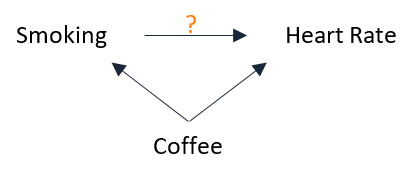
This diagram represents the following ideas:
- Coffee causes people to smoke, and not the other way around.
- Coffee causes an increase in heart rate.
Conclusion:
We should control for coffee in our study since it is a common cause of both smoking and heart rate — thus a confounding variable.
In the design phase:
We must collect information on whether a participant drinks coffee or not.
In the analysis phase:
We can control for coffee by including it as an independent variable in the following linear regression model:
Heart Rate = β0 + β1 Smoking + β2 Coffee
In this model, the coefficient β1 will reflect the effect of smoking on heart rate assuming a fixed amount of coffee consumed.
Adrenaline level as a potential confounder
Here’s a diagram that represents adrenaline level as a common cause of both smoking and heart rate:
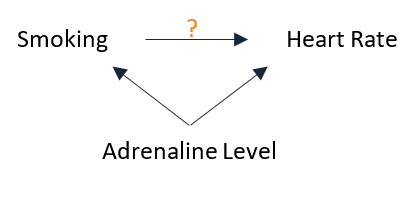
If this is the correct representation of the relationship between these 3 variables then:
- A high adrenaline level must cause an increase in heart rate.
- A high adrenaline level (representing a high level of stress) must also cause people to smoke, and not the other way around — i.e. smoking must not affect heart rate by increasing the level of adrenaline.
It is not clear whether this second part is true.
If not, then adrenaline level would be a mediator of the relationship between smoking and heart rate and not a confounder. And the diagram looks as follows:
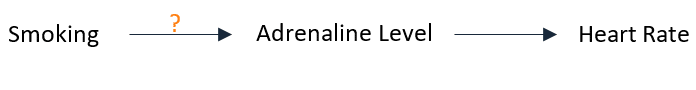
In this case, we should not control for adrenaline level in our analysis.
Why not?
Consider including the adrenaline level in our regression model:
Heart Rate = β0 + β1 Smoking + β2 Adrenaline
Then the coefficient β1 will reflect the effect of smoking on heart rate assuming a fixed adrenaline level. And since smoking acts on heart rate by increasing adrenaline, this model will be biased by showing a non-significant effect of smoking (i.e. β1 = 0).
Now let’s introduce another variable into our diagram: Stress.
Stress is a common cause of smoking and heart rate (indirectly by increasing adrenaline):
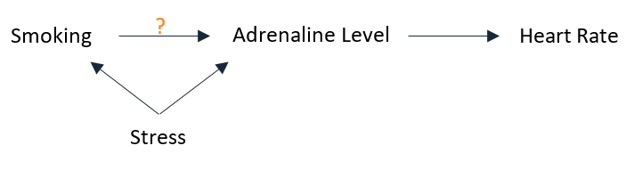
In this diagram, the relationship between smoking and heart rate is confounded by stress.
So the correct approach would be to adjust for stress (and not adrenaline level) by collecting some information about the stress level of the study participants (for instance, by using some validated questionnaire that detects stress).
Final model
Our analysis showed that we need to collect information from our sample on both coffee consumption and stress level, and adjust for them in our analysis.
Our final model must include 3 independent variables:
Heart Rate = β0 + β1 Smoking + β2 Coffee + β3 Stress
A simple linear regression model that does not include coffee and stress will not reflect the true effect of smoking on heart rate, instead it will reflect the effect of confounding from these variables.
Conclusion
The analysis of potential confounders should be done before collecting data for the study, since it will guide information collection.
In the words of a famous statistician:
To consult the statistician after an experiment is finished is often merely to ask him to conduct a post mortem examination. He can perhaps say what the experiment died of.
R.A. Fisher
Further reading
- 5 Real-World Examples of Confounding [With References]
- 4 Simple Ways to Identify Confounding
- 7 Different Ways to Control for Confounding
- Front-Door Criterion to Adjust for Unmeasured Confounding
- Why Confounding is Not a Type of Bias
- Using the 4 D-Separation Rules to Study a Causal Association
- List of All Biases in Research (Sorted by Popularity)