Confounding can be controlled in the design phase of the study by using:
- Random assignment
- Restriction
- Matching
Or in the data analysis phase by using:
- Stratification
- Regression
- Inverse probability weighting
- Instrumental variable estimation
Here’s a quick summary of the similarities and differences between these methods:
| Study Phase | Method | Can easily control for multiple confounders | Can control for unmeasured and unknown confounders | Can control for time-varying confounders |
|---|---|---|---|---|
| DESIGN | Random Assignment | YES | YES | YES |
| Restriction | NO | NO | NO | |
| Matching | NO | NO | NO | |
| DATA ANALYSIS | Stratification | NO | NO | NO |
| Regression | YES | NO | NO | |
| Inverse Probability Weighting | NO | NO | YES | |
| Instrumental Variable Estimation | YES | YES | NO |
In what follows, we will explain how each of these methods works, and discuss its advantages and limitations.
1. Random assignment
How it works
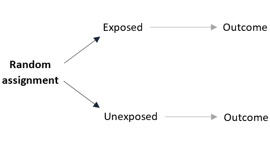
Random assignment is a process by which participants are assigned, with the same chance, to either receive or not a certain exposure.
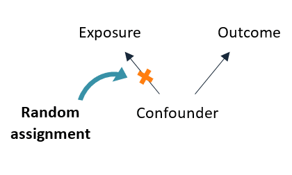
Randomizing the exposure adjusts for confounding by eliminating the influence of the confounder on the probability of receiving the exposure:
Advantage of random assignment:
Random assignment controls for confounding due to both measurable and unmeasurable causes. So it is especially useful when confounding variables are unknown or cannot be measured.
It also controls for time-varying confounders, that is when the exposure and the confounders are measured repeatedly in studies where participants are followed over time.
Limitation of random assignment:
Here are 3 reasons not to use random assignment:
- Ethical reason: Randomizing participants would be unethical when studying the effect of a harmful exposure, or on the contrary, when it is known for certain that the exposure is beneficial.
- Practical reason: Some exposures are very hard to randomize, like air pollution and education. Also, random assignment is not an option when we are analyzing observational data that we did not collect ourselves.
- Financial reason: Random assignment is a part of experimental designs where participants are followed over time, which turns out to be highly expensive in some cases.
Whenever the exposure cannot be randomly assigned to study participants, we will have to use an observational design and control for confounding by using another method from this list.
2. Restriction
How it works
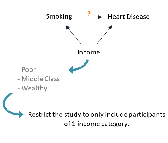
Restriction refers to only including in the study participants of a certain confounder category, thereby eliminating its confounding effect.
For instance, if the relationship between smoking (the exposure) and heart disease (the outcome) is confounded by income, then restricting our study to only include participants of the same income category will eliminate its confounding effect:
Advantage of restriction:
Unlike random assignment, restriction is easy to apply and also works for observational studies.
Limitation of restriction:
The biggest problem with restricting our study to 1 category of the confounder is that the results will not generalize well to the other categories. So restriction will limit the external validity of the study especially in cases where we have more than 1 confounder to control for.
3. Matching
How it works
Matching works by distributing the confounding variable evenly between the exposed and the unexposed groups.
The idea is to pair each exposed subject with an unexposed subject that shares the same characteristics regarding the variable that we want to control for. Then, by only analyzing participants for whom we found a match, we eliminate the confounding effect of that variable.
For example, suppose we want to control for income as a confounder of the relationship between smoking (the exposure) and heart disease (the outcome).
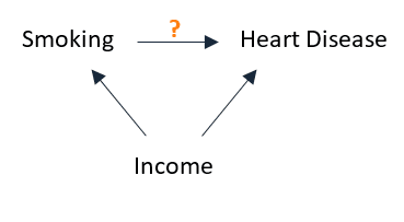
In this case, each smoker should be matched with a non-smoker of the same income category.
Here’s a step-by-step description of how this works:
Initially: The confounder is unequally distributed among the exposed and unexposed groups.
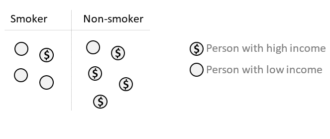
Step 1: Match each smoker with a non-smoker of the same income category.
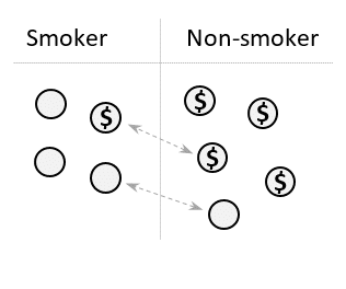
Step 2: Exclude all unmatched participants from the study.
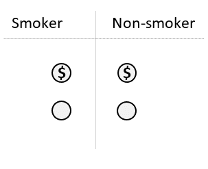
Result: The 2 groups will be balanced regarding the confounding variable.
Advantage of matching
Matching can be easy to apply in certain cases. For instance, matching on income in the example above can be done by selecting 1 smoker and 1 non-smoker from the same family, therefore having the same household income.
Limitation of matching
The more confounding variables we have to control for, the more difficult matching becomes, especially for continuous variables. The problem with matching on many characteristics is that a lot of participants will end up unmatched.
4. Stratification
How it works
Stratification controls for confounding by estimating the relationship between the exposure and the outcome within different subsets of the confounding variable, and then pooling these estimates.
Stratification works because, within each subset, the value of the confounder is the same for all participants and therefore cannot affect the estimated effect of the exposure on the outcome.
Here’s a step-by-step description of how to conduct a stratified analysis:
Step 1: Start by splitting the data into multiple subgroups (a.k.a. strata) according to the different categories of the confounding variable.
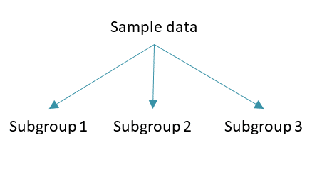
Step 2: Within each subgroup (or stratum), estimate the relationship between the exposure and the outcome.
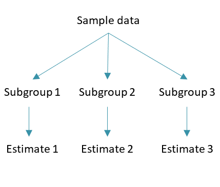
Step 3: Pool the obtained estimates:
- By averaging them.
- Or by weighting them by the size of each stratum — a method called standardization.
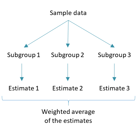
Result: The pooled estimate will be free of confounding.
Advantage of stratification
Stratified analysis is an old and intuitive method used to teach the logic of controlling for confounding. A more modern and practical approach would be regression analysis, which is next on our list.
Limitation of stratification
Stratification does not scale well, since controlling for multiple confounders simultaneously will lead to:
- Complex calculations.
- Subgroups that contain very few participants, and these will reflect the noise in the data more so than real effects.
5. Regression
How it works
Adjusting for confounding using regression simply means to include the confounding variable in the model used to estimate the influence of the exposure on the outcome.
A linear regression model, for example, will be of the form:
Outcome = β0 + β1 Exposure + β2 Confounder
Where the coefficient β1 will reflect the effect of the exposure on the outcome adjusted for the confounder.
Advantage of regression
Regression can easily control for multiple confounders simultaneously, as this simply means adding more variables to the model.
For more details on how to use it in practice, I wrote a separate article: An Example of Identifying and Adjusting for Confounding.
Limitation of regression
A regression model operates under certain assumptions that must be respected. For example, for linear regression these are:
- A linear relationship between the predictors (the exposure and the confounder) and the outcome.
- Independence, normality, and equal variance of the residuals.
6. Inverse probability weighting
How it works
Inverse probability weighting eliminates confounding by equalizing the frequency of the confounder between the exposed and the unexposed groups. This is done by counting each participant as many times as her inverse probability of being in a certain exposure category.
Here’s a step-by-step description of the process:
Suppose we want to control for income as a confounder of the relationship between smoking (the exposure) and heart disease (the outcome):

Initially: Since income and smoking are associated, participants of different income levels will have different probabilities of being smokers.
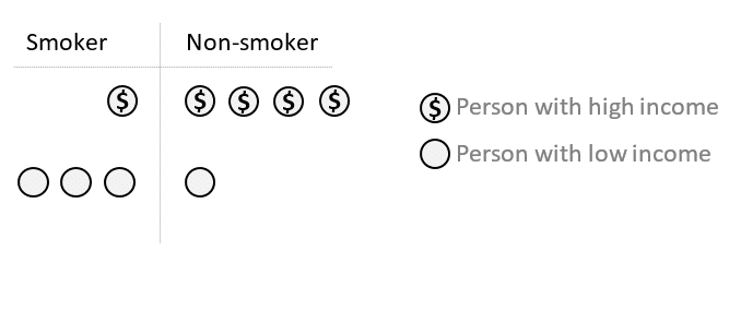
First, let’s focus on high income participants:
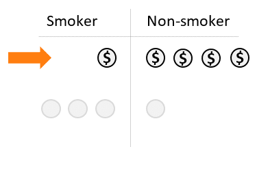
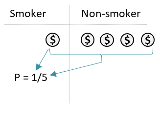
Step 1: Calculate the probability “P” that a person is a smoker.
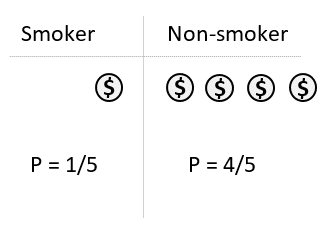
Step 2: Calculate the probability that a person is a non-smoker.
Step 3: Multiply each person by the inverse of their calculated probability. So each participant will no longer count as 1 person in the analysis. Instead, each will be counted as many times as their calculated inverse probability weight (i.e. 1 person will be 1/P persons).
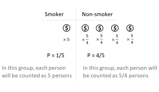
Now the smoking group has: 1 × 5 = 5 participants. And the non-smoking group also has: 4 × 5/4 = 5 participants
Finally, we have to repeat steps 1, 2, and 3 for participants in the low-income category.
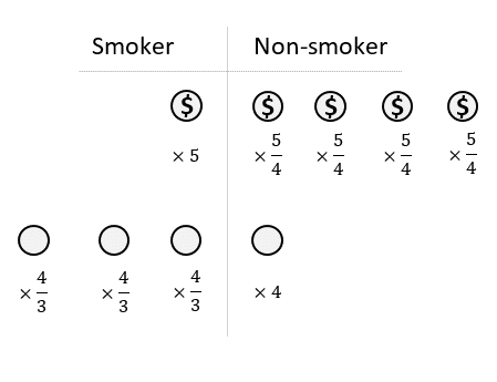
Result: The smoker and non-smoker groups are now balanced regarding income. So its confounding effect will be eliminated because it is no longer associated with the exposure.
Advantage of inverse probability weighting
This method is a type of what is referred to as G-methods that are used to control for time-varying confounders, that is when the exposure and the confounders are measured repeatedly in studies where participants are followed over time.
Limitation of inverse probability weighting
If some participants have very large weights (i.e. when their probability of being in a certain exposure category is very low), then each of these participants would be counted as a large number of people, which leads to instability in the estimation of the causal effect of the exposure on the outcome.
One solution would be to exclude from the study participants with very high or very low weights.
7. Instrumental variable estimation
How it works
The instrumental variable method estimates the unconfounded effect of the exposure on the outcome indirectly by using a variable — the instrumental variable — that represents the exposure but is not affected by confounding.
An instrumental variable satisfies 3 properties:
- It causes the exposure.
- It does not cause the outcome directly — it affects the outcome only through the exposure.
- Its association with the outcome is unconfounded.
Here’s a diagram that represents the relationship between the instrumental variable, the exposure, and the outcome:
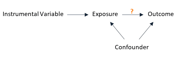
An instrumental variable is chosen so that nothing appears to cause it. So in a sense, it resembles the coin flip in a randomized experiment, because it appears to be randomly assigned.
How the instrumental variable can be used to study causality?
Looking at the data, if an association is found between the instrumental variable and the outcome then it must be causal, since according to property (3) above, their relationship is unconfounded. And because the instrumental variable affects the outcome only through the exposure, according to property (2), we can conclude that the exposure has a causal effect on the outcome.

So how to quantify this causal/unconfounded effect of the exposure on the outcome?
Let “α1” denote the magnitude of the causal effect of the instrumental variable on the exposure, and “β1” that of the exposure on the outcome.
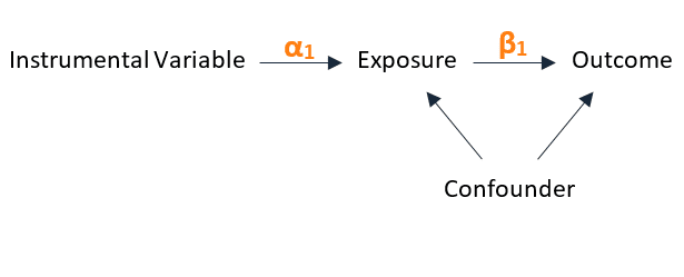
So our objective is to find β1.
Note that the simple regression model between the exposure and the outcome produces a confounded estimate of β1:
Outcome = β0 + β1 Exposure
And therefore does not reflect the true β1 that we are searching for.
So how to find this true unconfounded β1?
Technically, if we think in terms of linear regression:
- α1 is the change in the exposure CAUSED by a 1 unit change in the instrumental variable.
- β1 is the change in the outcome CAUSED by a 1 unit change in the exposure.
It follows that a 1 unit change in the instrumental variable CAUSES an α1 × β1 change in the outcome (since the instrumental variable only affects the outcome through the exposure).
And as discussed above, any association between the instrumental variable and the outcome is causal. So, α1 × β1 can be estimated from the following regression model:
Outcome = a0 + a1 Instrumental_Variable
Where a1 = α1 × β1
And because any association between the instrumental variable and the exposure is also causal (also unconfounded), the following model can be used to estimate α1:
Exposure = b0 + b1 Instrumental_Variable
Where b1 = α1
We end up with 2 equations:
- α1 = b1
- α1 × β1 = a1
A simple calculation yields: β1 = a1/b1 which will be our estimated causal effect of the exposure on the outcome.
Advantage of instrumental variable estimation
Because the calculations that we just did are not dependent on any information about the confounder, we can use the instrumental variable approach to control for any measured, unmeasured, and unknown confounder.
This method is so powerful that it can be used in cases even where we do not know whether there is confounding or not between the exposure and the outcome, and which variables are suspect.
Limitation of instrumental variable estimation
In cases where the instrumental variable and the exposure are weakly correlated, the estimated effect of the exposure on the outcome will be biased.
The use of linear regression is also constrained by its assumptions, especially linearity and constant variance of the residuals.
As a rule of thumb, use the instrumental variable approach in cases where there are unmeasured confounders, otherwise, use other methods from this list since they will, in general, provide a better estimate of the causal relationship between the exposure and the outcome.
If you are interested, here are 3 Real-World Examples of Using Instrumental Variables.
References
- Hernán M, Robins JM. Causal Inference. Chapman & Hall/CRC; 2020.
- Roy J. A Crash Course in Causality: Inferring Causal Effects from Observational Data | Coursera.
- Pearl J, Mackenzie D. The Book of Why: The New Science of Cause and Effect. First edition. Basic Books; 2018.