Linear regression assumes that the dispersion of data points around the regression line is constant.
We can deal with violation of this assumption (i.e. with heteroscedasticity) by:
- Transforming the outcome variable
- Calculating heteroscedasticity-robust standard errors
- Using weighted regression
- Using a t-test with unequal variances (when dealing with only 1 categorical predictor)
- Converting the outcome into a binary variable then using logistic regression
Let’s create some heteroscedastic data to demonstrate these methods:
set.seed(0)
x = runif(100)
y = x + rnorm(n = 100, mean = 10, sd = x)

model = lm(y ~ x)

# plot residuals vs fitted values
plot(model, 1, pch = 16)
Output:
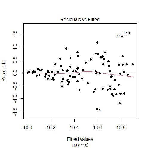
The residuals vs fitted values plot shows a fan shape, which is evidence of heteroscedasticity. (For more information, see: How to Check Linear Regression Assumptions in R)
Solution #1: Transforming the outcome variable
The first solution we can try is to transform the outcome Y by using a log or a square root transformation.
The difference is that with a log transformation the model will still be interpretable, so this is what we are going to use here (for information on how to interpret such model, see: Interpret Log Transformations in Linear Regression):
model1 = lm(log(y) ~ x)

# re-check residuals vs fitted values plot
plot(model1, 1)
Output:
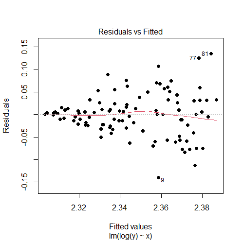
The log transformation did not solve our problem in this case since the residuals vs fitted values plot is still showing a fan shape instead of a random pattern.
Solution #2: Calculating heteroscedasticity-robust standard errors
Since heteroscedasticity only biases standard errors (and not regression coefficients), we can replace them with ones that are robust to heteroscedasticity.
Here’s how to do it in R:
model = lm(y ~ x)

library("lmtest") # for coeftest
library("sandwich") # for vcovHC

# estimating heteroscedasticity-robust standard errors
coeftest(model, vcov = vcovHC(model))
Output:
t test of coefficients:

            Estimate Std. Error  t value  Pr(>|t|)
(Intercept) 9.986870   0.073587 135.7143 < 2.2e-16 ***
x           0.920409   0.193715   4.7514 6.922e-06 ***
---
Signif. codes:  0 ‘***’ 0.001 ‘**’ 0.01 ‘*’ 0.05 ‘.’ 0.1 ‘ ’ 1
In this case, the robust standard errors differed a little bit from the ordinary standard errors calculated using summary(model).
Solution #3: Using weighted regression
Another solution would be to use weighted regression where we handle heteroscedasticity by imposing less weight on the part of the data where the variance is high, and more weight on the part where the variance is low.
How to calculate the weights for weighted regression?
First of all, these weights should be inversely proportional to the variance of Y, so:
weights = 1/variance of Y
Next, we will have to guess the variance of Y for different values of X. Our best guess of this variance is to regress the absolute values of the residuals against the fitted values. The resulting fitted values squared of this regression will be our estimates of this variance. (For more information, see Weighted Regression)
In R we run the following code:
# ordinary linear regression model
model = lm(y ~ x)

# estimating the variance of y for different values of x
variance = lm(abs(model$residuals) ~ model$fitted.values)$fitted.values^2

# calculating the weights
weights = 1 / variance

# weighted regression model
weighted_model = lm(y ~ x, weights = weights)
summary(weighted_model)
Output:
Call:
lm(formula = y ~ x, weights = weights)

Weighted Residuals:
    Min      1Q  Median      3Q     Max
-3.0384 -0.9777  0.0516  0.6491  3.4628

Coefficients:
            Estimate Std. Error t value Pr(>|t|)
(Intercept) 10.00850    0.02994 334.282  < 2e-16 ***
x            0.86790    0.11637   7.458 3.57e-11 ***
---
Signif. codes:  0 ‘***’ 0.001 ‘**’ 0.01 ‘*’ 0.05 ‘.’ 0.1 ‘ ’ 1

Residual standard error: 1.207 on 98 degrees of freedom
Multiple R-squared:  0.3621,	Adjusted R-squared:  0.3556
F-statistic: 55.62 on 1 and 98 DF,  p-value: 3.57e-11
Solution #4: Using a t-test with unequal variances
When we are dealing with only 1 categorical predictor, we can use a t-test with unequal variances (a.k.a. Welch’s t-test) instead of linear regression to estimate the relationship between x and y:
t.test(x, y) # the default is to run a Welch's t-test
Output:
	Welch Two Sample t-test

data:  x and y
t = -159.43, df = 142.38, p-value < 2.2e-16
alternative hypothesis: true difference in means is not equal to 0
95 percent confidence interval:
 -10.068735  -9.822109
sample estimates:
 mean of x  mean of y
 0.5207647 10.4661865
Solution #5: Converting the outcome into a binary variable then using logistic regression
This is the least favorable solution, since converting a continuous variable into binary involves losing information.
The cutpoint to split the y variable should be chosen according to background knowledge. In the example below, we will split y in half using its median as a cutpoint:
y_binary = as.factor(ifelse(y > median(y), 'high', 'low'))

# run logistic regression
summary(glm(y_binary ~ x, family = 'binomial'))
Output:
Call:
glm(formula = y_binary ~ x, family = "binomial")

Deviance Residuals:
     Min        1Q    Median        3Q       Max
-1.61361  -0.95142  -0.01876   0.89945   1.84797

Coefficients:
            Estimate Std. Error z value Pr(>|z|)
(Intercept)   2.0157     0.5327   3.784 0.000155 ***
x            -3.8594     0.9217  -4.187 2.82e-05 ***
---
Signif. codes:  0 ‘***’ 0.001 ‘**’ 0.01 ‘*’ 0.05 ‘.’ 0.1 ‘ ’ 1

(Dispersion parameter for binomial family taken to be 1)

    Null deviance: 138.63  on 99  degrees of freedom
Residual deviance: 116.96  on 98  degrees of freedom
AIC: 120.96

Number of Fisher Scoring iterations: 4
If you are interested, see: How to Run and Interpret a Logistic Regression Model in R.